Imagine has had support for Catmull-Clark subdivision of quads within its interface for a while now, but the previous implementation had several limitations: it was slow and memory-inefficient (it just brute-forced the subdivision from the original faces), it didn’t support open shapes with holes and it didn’t keep UVs.
I’ve now re-written this to use a half-edge mesh structure, which makes it faster (less duplicate work is done), it supports boundary edges (holes in geometry), supports triangles and it subdivides UV positions (linearly at preset). I’ve also added support for linear subdivision with no smoothing.
Once I sort out the Geometry Instance infrastructure for each object in order to allow Geometry Modifiers at render time, it should be fairly simple to add Displacement support.
Discussion at work led to talking about implementing a wireframe shader in Nuke, so I decided to see how difficult
it would be in Imagine. As long as the mesh consists of polygons of a single type - i.e. triangles or
quads: not difficult at all it turns out.
For triangles, it’s easy enough to emulate a wireframe surface by simply working out how close a hit position
on a triangle is to an edge by transforming the triangle’s points into world space and then using the standard
point-to-line method of a perpendicular vector to each edge. This gives you the distance in world space of the
hit position to each edge, and based on which distance is the closest, you can then apply a step function to
the colour of the surface, based on the distance and a line thickness amount.
For quads, I first tried using the same algorithm as for triangles, but ignoring the edge of the triangle that was
shared within the quad. This worked to some degree, but each quad had two opposing wedges in the corners where the
point-to-line formula meant that parts of some edges weren’t shaded correctly.
So instead, I decided to use the Barycentric coordinates of the hit position within the triangle. This allowed me to correctly isolate all four edges of the quad based on a fixed threshold, but I then had to work out the line width and keep it uniform to the length of any edges. In the end I multiplied the Barycentric coordinates of both the the hit position and the inverse hit position (for the opposing edge of the quad) by the length of each of the non-shared edges of the triangle, giving a distance. The smallest of these distances I then used to step the colour, as I did for triangles. While this might not be perfectly accurate and work in all situations, it seems to work very well in practice and also allowed me to (almost) match the line thickness to the triangle method. It also looks very nice:
There’s a very slight (~1%) overhead in shading, as triangles have to be fetched and transformed to world space, but both of the renderings above at full HD finished in under six minutes with 676 samples per pixel.
When I sort out the texturing infrastructure to make it more flexible, it should be very easy to apply this texture as an alpha texture for a fully-3-dimensional mesh that is able to be seen through and cast shadows.
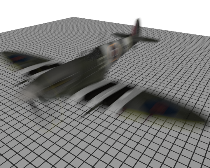
After recently trying to render an animation with Imagine, the result consisting of heavy aliasing in the form of walking and flickering edges on small objects, I realised that I couldn’t put off adding proper Reconstruction Filtering to Imagine any longer.
With no filtering, each sample which contributes to a pixel’s final colour has equal weighting to the final result, which leads to heavy aliasing as objects move across the frame. Using Reconstruction Filtering, the sample’s weighting to the final result is related to its distance from the centre of the pixel.
There are many different kinds of filters that can be used for Reconstruction Filtering, ranging from Box filtering (which is the same as no filtering - at least with a default filter width of 1), Gaussian (smooth, slightly blurred) to Lanczos Sinc (very sharp, having negative lobes). Unfortunately, no filter is perfect for every scenario, although generally for stills, you can get away with sharper filters.
I’ve implemented Triangle, Gaussian and Mitchell Netravali filters currently, which along with Box (no filtering) you can see enlarged examples of below:
I’ve been doing a lot of back-end work to Imagine recently, with no new obvious features to show in terms of output images, but a thorough refactoring of some of the core code. I’ve also added remote rendering support, Deep Image (OpenEXR 2) output, adaptive rendering and refinement-progressive rendering.
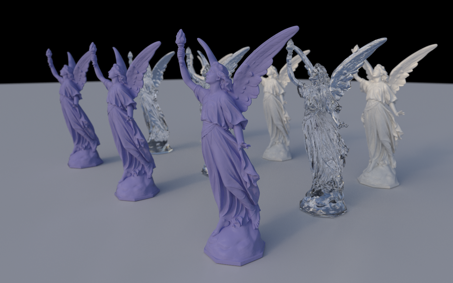
Imagine has had support for instanced geometry since very early on, so this is nothing new, but I’ve added to the interface the ability to create instance copies in the shape of other mesh shapes, which shows off the feature more impressively.
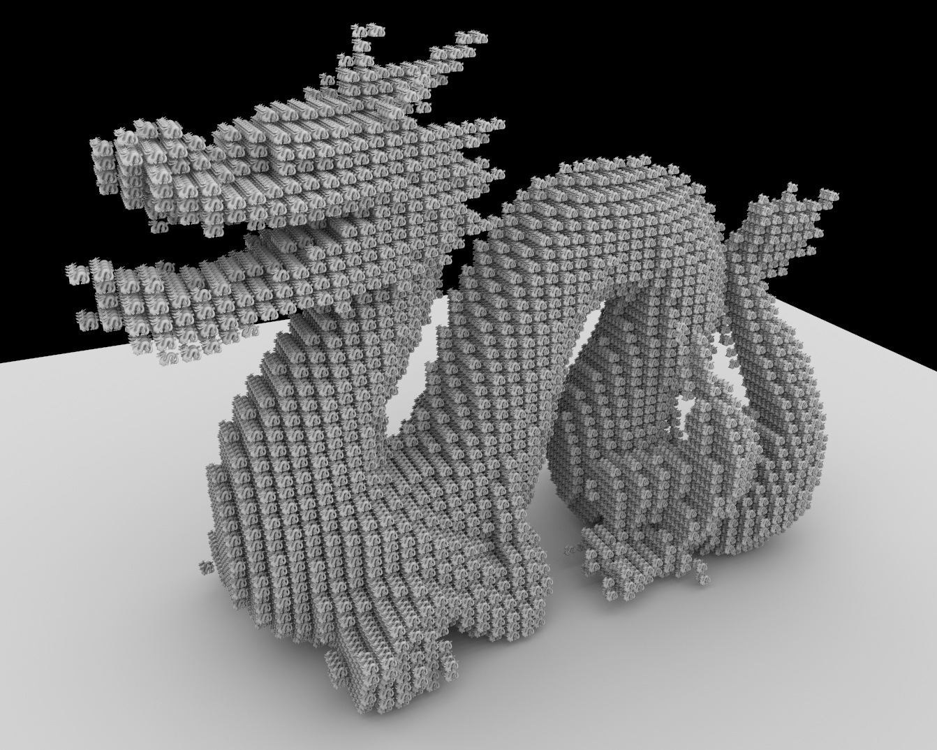
At some point, it would be nice to have a look at adding support for recursive procedurals like Katana supports, for infinite scenes (dragons made up of dragons, made up of dragons, etc, etc.)
I finally got the transformation infrastructure sorted out in order to facilitate adding transformation motion blur support to Imagine. Each ray sample per-pixel has a stratified time sample over the shutter’s open duration. There’s a bit of overhead, as each ray (if it hits the expanded boundary box of the objects bounds for the shutter time) has to interpolate the object’s transform matrix for its time delta.
In addition, as with depth-of-field circle-of-confusion sampling, care has to be taken so that the samples don’t interfere/correspond too closely with the camera’s pixel sample positions, otherwise aliasing occurs. Randomly shuffling the positions seems to do quite nicely.
The majority of the time spent when raytracing is generally intersecting rays with the scene and the objects in the scene. The two main ways to reduce the time taken to raytrace scenes are to either reduce the cost of each ray intersection (by using acceleration structures), or to send less rays.
Sending less rays obviously has a direct impact on the speed of rendering the scene, but care has to be taken to make sure image quality doesn’t suffer as a result: normally more samples per-pixel are used in order to reduce the noise (or variance) in an image. There are a variety of techniques that can be used to maximise the effectiveness of the rays sent out into the scene from adaptive super-sampling (sending out more rays per-pixel when the samples within the pixel are dissimilar) to efficient sampling (by ensuring that there’s a good distribution of samples across all sampling dimensions) through to importance sampling.
Importance Sampling is a technique whereby samples are selected so that a variable that has the most effect on the variance of the overall end result has the most distribution.
An excellent example of this is with environment lighting - if we use the following environment map for lighting a scene:
there are only two very small areas of illumination coming from the map. Without using importance sampling - by randomly sampling locations from the map - there is a low probability that any of the samples will actually correspond to the two coloured dots on the texture map. This means that either the image will be too dark (and won’t evaluate the two coloured dots correctly), or there will be very high variance where a few samples that sample the light pick up one of the coloured spots, but most don’t. This will result in extreme noise, as can be seen in this render without importance sampling:
With importance sampling, it is possible to build up a two-dimensional map of importance based on the corresponding luminance of the environment map, which allows any light sample for the environment map to map to an actual position on the texture map where there is colour - i.e. one of the two coloured spots. The weighting of the function has to be modified as well, in order to not bias the equation (by assuming that the entire image is yellow and blue with no black) which would give unrealistic results.
The final result with importance sampling can be seen below:
Both images were rendered with 32 samples per-pixel, and the noise-reduction importance sampling gives in this case is striking.
The ideal situation in terms of efficiency for a raytracer when tracing rays around a scene is that the acceleration structures take the brunt of the work (assuming a simple use-case with no complex shading, displacement/subdivision or asset paging) - that is, if you profile the raytracer, the acceleration structure intersection functions are being hit more than the actual intersection functions of the primitives within the acceleration structures. This depends on quite a few things, like the layout of the scene, the acceleration structure, the geometry and how tightly boundary boxes (of either the object or any the acceleration structures use) fit around geometry or other areas.
There’s a balancing point between the density of the geometry being intersected against and how efficient the acceleration structure being used is. With a KDTree (and to a lesser extent with BVH or BIH), this is generally governed by the depth of the acceleration structures. With a Grid acceleration structure, this is done by the number of grid cells the scene area or mesh is covered by. Up to a certain point (and assuming the acceleration structure works well) increasing either of these variables increases the efficiency of the overall ray intersection process, as in ideal situations (generally most of the time), this allows less intersection tests to be needed, because the cells of the acceleration structure storing the primitives store less primitives, so less primitives have to be tested against the ray. However, increasing these numbers comes at a price - the build time of the acceleration structure goes up, as does the amount of memory required to store it. In the KDTree’s case, both of these can quite quickly become prohibitive.
Something that is common with acceleration structures (especially KDTrees, Grids and BIHs) is the fact that primitives within the acceleration structure can often be in multiple nodes or cells at once if they straddle the boundary. Due to the way most ray traversal algorithms work with the respective acceleration structures, they generally involve walking the ray through the structure until it finds nodes or cells with primitives in, and then testing each primitive in that node/cell against the ray. In the case when a ray didn’t intersect with any primitives in one node/cell and so the ray moves to the next node/cell, if some of the primitives in this next node were in the previous node as well, they will have already been intersected against the ray, so they’re not going to intersect that primitive this time. This can be quite wasteful.
In A fast voxel traversal algorithm for raytracing, J. Amanatides and A. Woo introduced a method to avoid this inefficiency, whereby each ray and each primitive have a unique ID, and when a ray is intersected against a primitive, a 2D matrix is marked with the respective ray and primitive IDs, so that a fast lookup can be done in the future to skip the test if the situation arises again. This works very nicely when there are a few number of rays (e.g. only one for physics collision tests or similar) or when there are a fairly low number of primitives and rays. But when the number of primitives and rays are both in the millions, then the amount of memory required to store this matrix becomes ridiculous, not to mention causing huge CPU cache latency problems (due to cache misses), which significantly outweigh any benefit that using the technique might provide.
In Realtime Ray Tracing on Current CPU Architectures, C. Benthin introduced (section 4.4.4) the “Hashed Mailbox”, whereby, because for a particular ray intersection test (assuming a fairly good acceleration structure) the ray will only have to be intersected against a small subset of the total number of primitives that exist, a much smaller amount of memory is actually required in order to still give a useful efficiency boost. So a small amount of memory (with around 64 slots) is allocated, and the slots to use for marking primitives that have been checked are selected based on hashing the primitive ID. This gave on average between 15% to 25% speed increases. This new technique still requires a fair amount of memory (1KB) to be allocated and freed however, which can itself still have an overhead, especially if it is done on a per-ray-intersection basis.
In Ray-triangle intersection algorithm for modern cpu architectures, A. S. Maxim Shevtsov and A. Kapustin introduced “Inverse Mailboxing”, which uses even less memory (32 bytes for an 8-mailbox slot structure), which simply stores the last eight intersected objects on the stack, and so can be easily used within the ray traversal code/algorithm. This method doesn’t guarantee that duplicate object intersection tests will not be made per-ray for any object, but assuming a decent acceleration structure and a limited number of primitives per node or cell, the chances of duplicate checks will be very small, while still providing a useful speedup.
I’ve found using this last technique has for general meshes given between 7%-23% speedups, and in the case of compound objects (objects with sub-objects within them) - where the cost of intersecting the sub-objects can be much more expensive than just a simple primitive intersection - up to a 40% speed increase.
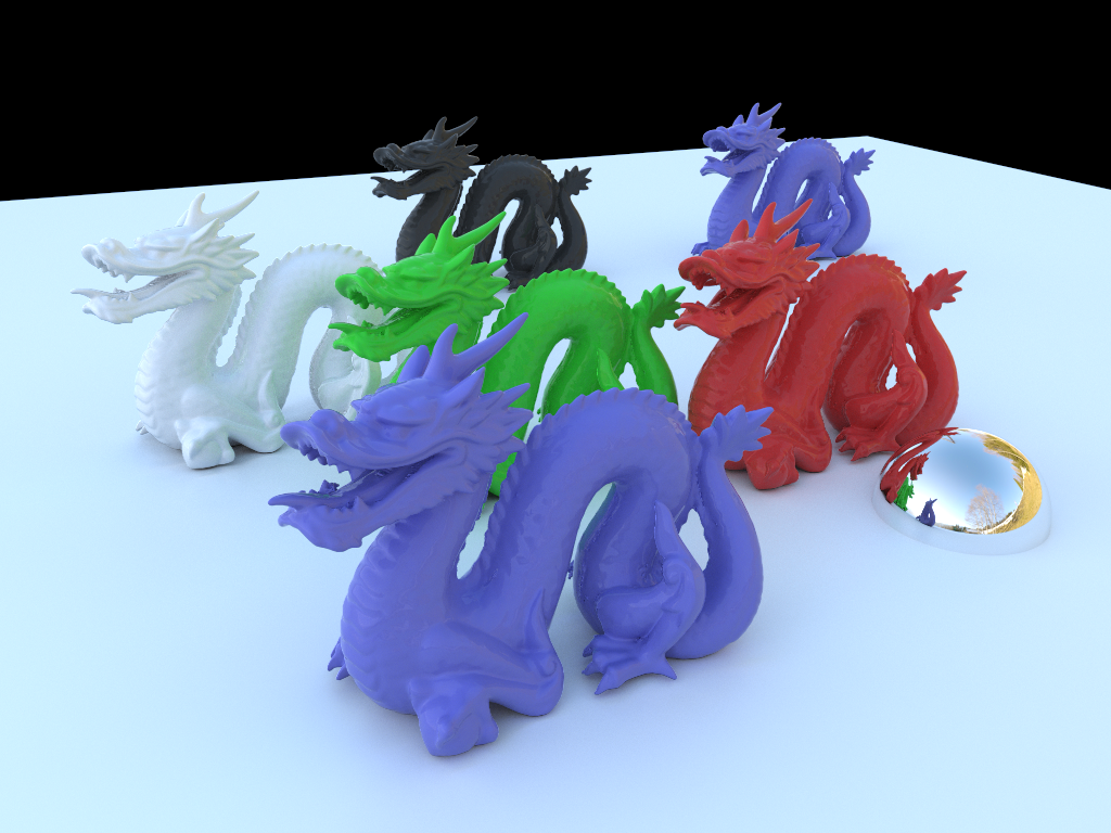
Showcasing an environment light - with no really intense illumination areas, hence the very diffuse
shadows - and a selection of different coloured dragons in a metallic paint material (a varnishy paint layer
on metal), including dielectric reflection, a dielectric layer with a diffuse BSDF and a microfacet-based dielectric layer.
Importance sampling still needs to be added to the environment light, so a large number of samples are needed to reduce the noise.