This month I bought and received a new Apple MacBook Pro (M2 Pro, 14-inch, 2023) with the aim of replacing my own Apple MacBook Pro 15-inch (Intel) 2015 model which I bought in 2016. The MacBook Pro 15 still does work, but the battery life is awful now (I could have it replaced, which I’ve done several times with laptops in the past), the internal fans barely work, and the rubber around the screen is disintegrating, so with a trip back to the Northern Hemisphere planned next month, I thought it was time for a replacement.
A year ago I was provided (on loan) a work-provided MacBook Pro 14 M1 Pro (see previous benchmarks) which I’ve been using a bit, so I knew mostly what to expect in terms of performance and from the laptop in general, but I was curious to compare the performance of the M2 Pro against the M1 Pro (and the old Intel machine).
It’s not going to be a completely fair apples-to-apples comparison, as the work-provided MacBook Pro 14 M1 Pro processor is the 10-core version which has two extra performance cores than the baseline did - having eight performance cores and two efficiency cores - and the M2 Pro I’ve just bought is the baseline model - with six performance cores and four efficiency cores - but it should provide a rough indication of what performance to expect.
The Xcode / Apple Clang compiler versions are also different: My MacBook Pro 15 (Intel) is still running quite an old MacOS version, with an older compiler which I don’t want to update, and while I did install Xcode 14.3 on the 2021 MacBook Pro M1 Pro (as well as the command line tools) in order to attempt to match what I’d just installed on my new 2023 MacBook Pro M2 Pro, clang --version still shows version 13.1.6, whereas my new 2023 M2 Pro MacBook Pro shows 14.0.3 being used, so I’m not really sure what’s going on there, as Xcode -> About Xcode shows Version 14.3.1 as I’d expect on both MacBook Pro 14 machines (and both have the command line tools for that version of Xcode installed).
The MacBook Pro 14s are both running MacOS Ventura 13.4.
Tests:
Copying what I did in the test last year, I’ll be using two of my apps as benchmarks: my Mint interpreter language VM (originally based off Robert Nystrom’s excellent Crafting Interpreters Lox language tutorial) but with additional functionality and performance improvements, which I’ll use to benchmark two Mint scripts as single-threaded tests, and also my Imagine pathtracing renderer, which has native SSE intrinsics support for Intel and native Neon intrinsics support for ARM, which I’ll run in both single- and multi-threaded scenarios.
Both apps will be compiled with -march=native on the Intel side and -mcpu=native on the Apple Silicon / ARM side, using the clang version on the machine in question, as well as optimisation level: -O3.
The two Mint script tests will be loop value calculation as Test 1:
var a = 1;
for (var i = 0; i < 100000000; i += 1)
{
    a = (i + i + 3 * 2 + i + 1 - 0.42) / a;
}
print a;
and a variation of Project Euler 21 to calculate the sum of all Amicable numbers under 15,000 as Test 2.
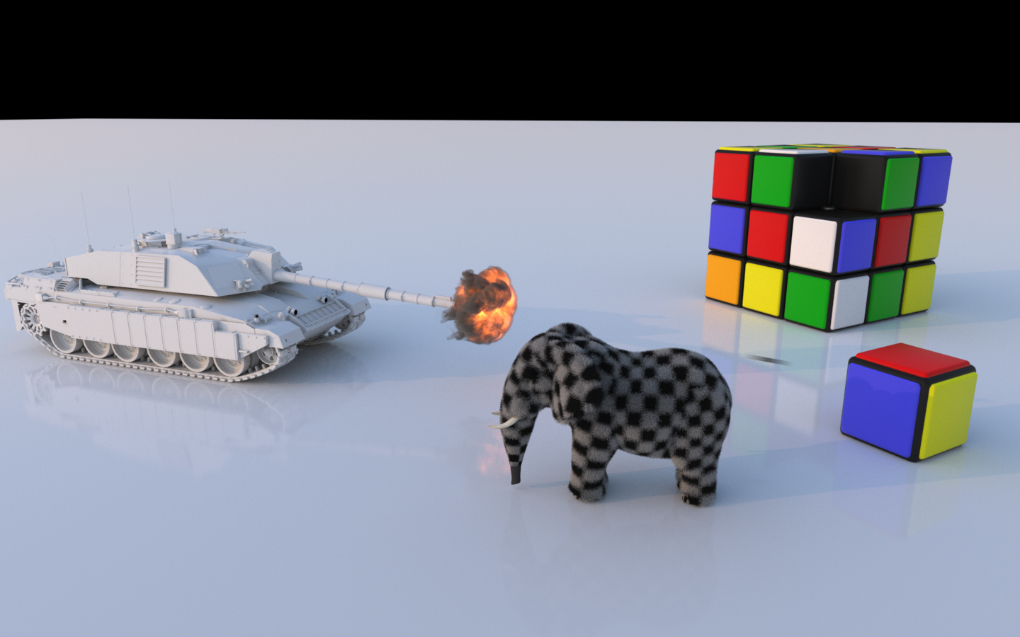
The Imagine rendering tests will render three different scenes in both single- and multi-threaded mode.
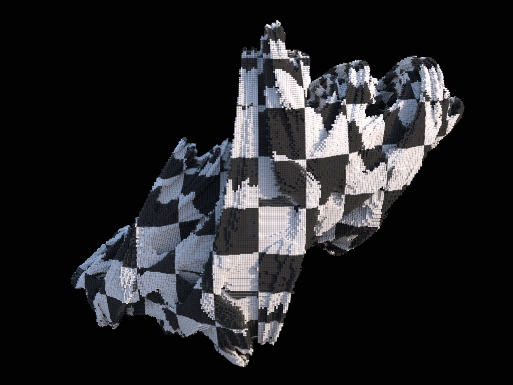
The first render will be the same maze scene with spherical area lights that I used in the test last year (example image above), but with different settings:
resolution will be 256 x 256, 256 samples-per-pixel will be used, but this time only one next-event light sample will be taken each path vertex.
The general ray traversal and ray intersection will utilise SIMD, but the (fairly expensive) perfect light sphere sampling is scalar, and very unlikely
to be vectorised by the compilers themselves.
The second render will be a 450 x 338 resolution render of a Signed Distance Field primitive of a Julia Fractal (example image above, although with different settings), which is quite expensive to evaluate,
and also does not have any SIMD utilisation for the SDF evaluation / intersection. There’s a physical Sky IBL in the scene as a light, and 144 samples-per-pixel will be used, with 3x3 Blackman Harris pixel filtering being used.
The third render will be a 450 x 338 resolution render of 2,326,299 instanced mesh cubes in the (pre-calculated) shape of a Julia Fractal, which will
fully-utilise SIMD instructions for ray traversal in the BVH and for ray / primitive intersections. Again, there’s a physical Sky IBL in the scene,
144 samples-per-pixel will be used, but this time no pixel reconstruction filtering will be used (so effectively Box 1x1).
These tests will all be done on (close to fully-charged) battery power - I discovered in the tests last year that Apple doesn’t seem to down-clock on battery power - and I will also wait between test runs for the processor temperatures to be below 50 degC before running the next test, to try and reduce the impact of thermal throttling.
All tests will be run three times, and results below will show the mean average of those numbers.
Results
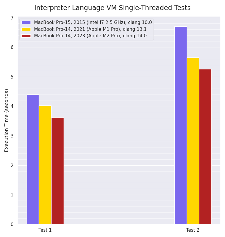
Single-threaded Mint VM interpreter:
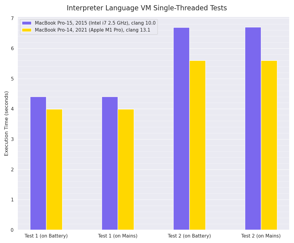
Single-threaded Mint interpreter VM benchmarks, smaller values are better:
For these single-threaded tests, the M2 Pro has a small improvement over the M1 Pro’s performance, which itself is around 10-16% faster than the eight year old Intel i7 processor. As mentioned last year however, I think this is very likely because the Mint VM execution is often branch-prediction constrained within the main VM bytecode interpreter loop, so there’s a limit to the amount of Instruction-Level Parallelism that’s achievable from the eight-wide M1 Pro and M2 Pro.
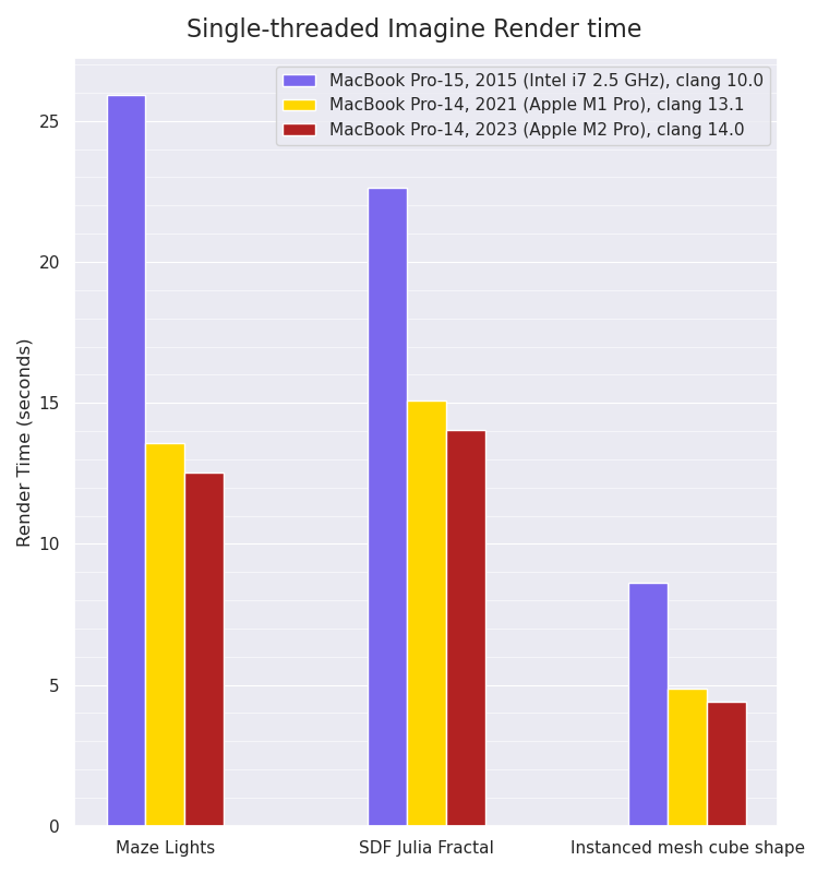
Single-threaded Imagine rendering:
Single-threaded Imagine rendering benchmarks, smaller values are better:
The single-threaded rendering tests, which have a lot more floating point calculations and SIMD usage, show a small performance improvement for the M2 Pro over the M1 Pro. Intriguingly, the Maze Lights scene is the test with the biggest performance increase (almost 2x faster) from the Intel machine to the Apple M1 Pro: the other tests show slightly smaller gains, which I wouldn’t have expected. Without further microbenchmarks of various isolated parts of those tests, it’s difficult to guess why that might be, but the different render tests do exercise different calculations and code paths.
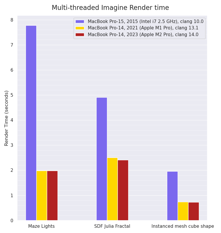
Multi-threaded Imagine rendering:
Multi-threaded Imagine rendering benchmarks, smaller values are better:
The multi-threaded rendering tests show that due to the fact the M1 Pro machine has eight performance cores and two efficiency cores, whilst the M2 Pro
machine only has six performance cores and four efficiency cores, the M2 Pro machine is only very slightly faster in the SDF Julia Fractal render scene than the M1 Pro machine, and ties in the other two tests. Once again, the Maze Lights scene shows the biggest performance increase - almost 4x faster - from the Intel CPU to the Apple Silicon ones, with the other two tests showing a less dramatic difference (between 2x to 3x faster).
Conclusion
I think a not too bad showing for the baseline model: the M2 Pro can beat the M1 Pro by a small margin in all single-threaded tests, and can either just about equal or slightly beat the M1 Pro which has more performance cores (but two less efficiency cores) in the multi-threaded tests.
Last week I received a work-provided (on loan) new Apple MacBook Pro (14-inch, 2021) with the Apple M1 Pro 10-core processor, so I was very curious to see how it performed with some of my code, given the generally excellent reviews and reports I’d seen by people with it online.
I have my own MacBook Pro 15-inch 2015 (Intel i7) model which I’ll be comparing it against as a basic benchmark performance test, although it won’t be a completely fair test as the two machines are running different versions of MacOS and the clang compiler, and I didn’t want to upgrade my own machine’s MacOS version to a newer version (for various reasons). So the code being executed on the different machines will be generated by different versions of clang, but given the micro-architecture is totally different anyway, I think it’s still a meaningful test and at least will show the performance difference between the two laptops.
My old MacBook Pro 15-inch 2015 is a 2.5 GHz Intel Core i7, with four cores, eight threads, and 1600 Mhz DDR3 memory, running macOS 10.14.5 (Mojave), with Xcode 10.2.1 installed which has clang version 10.0.1.
The new MacBook Pro 14-inch 2021 is the M1 Pro 10-core version, with 8 performance cores and 2 efficiency cores, running macOS 12.3 (Monterey), with Xcode 13.4.1 installed which has clang version 13.1.6.
Tests:
I’ll be using two of my apps as benchmarks: my Mint interpreter language VM (originally based off Robert Nystrom’s excellent Crafting Interpreters Lox language tutorial) but with additional functionality and performance improvements, which I’ll use to benchmark two Mint scripts as single-threaded tests, and also my Imagine pathtracing renderer, which has native SSE intrinsics support for Intel and native Neon intrinsics support for ARM, which I’ll run in both single- and multi-threaded scenarios.
Both apps will be compiled with -march=native on the Intel side and -mcpu=native on the Apple M1 Pro ARM side, using the clang version on the machine in question, as well as optimisation level: -O3.
The two Mint script tests will be loop value calculation as Test 1:
var a = 1;
for (var i = 0; i < 100000000; i += 1)
{
    a = (i + i + 3 * 2 + i + 1 - 0.42) / a;
}
print a;
and a variation of Project Euler 21 to calculate the sum of all Amicable numbers under 15,000 as Test 2.
The Imagine rendering tests will render the below example scene of a basic maze with 12 spherical area lights and one hemisphere light, with four Next Event Estimation samples being taken each bounce to evaluate the lighting, and using Cone sampling to perfectly sample each spherical area light from each hitpoint, with 256 samples-per-pixel being done, using stratified sampling and a ray depth of 6 diffuse bounces. Depending on the setup of the tests (single-threaded, multi-threaded, etc), I’ll render the scene at resolutions of: 150 x 150, 300 x 300 and 600 x 600.
For all tests, I’ll run them on battery power and then mains power, in case that affects the clocking of the processors, and will also wait between test runs for the processor temperatures to be below 50 degC before running the next test, to try and reduce the impact of thermal throttling. However, for the longer-running multi-threaded Imagine rendering tests I’m fairly sure thermal throttling will start to take place on the Intel 2015 machine given how fast the fans start to spin in longer-running scenarios.
All tests will be run three times, and results below will show the mean average of those numbers.
Results
Single-threaded Mint VM interpreter:
Single-threaded Mint interpreter VM benchmarks, smaller values are better:
For these single-threaded tests, the M1 Pro has fairly modest (~11% faster in Test 1, ~16% faster in Test 2) improvements over the seven year old Intel i7, however as the Mint VM execution is often branch-prediction constrained within the main VM bytecode interpreter loop, I expect this doesn’t really allow the M1 Pro’s eight-wide design to really stretch its legs running these benchmarks, as there’s a limit to the amount of Instruction-Level Parallelism that’s achievable.
It’s interesting to see that there’s no apparent difference in performance between running on battery vs running connected to the mains: I was expecting to see a difference - even if only on the Intel i7 MBP - as I know my Thinkpad T480s running Linux shows significant performance differences between the two states, but Apple clearly don’t seem to be implementing that strategy.
Single-threaded Imagine rendering:
Single-threaded Imagine rendering benchmarks, smaller values are better:
Things start to look more impressive for the M1 Pro in the single-threaded rendering tests, as here there are a lot more floating point calculations being done with a lot less branching, and there’s a fair amount of SIMD use (i.e. ray intersection / traversal code, which uses native SSE or Neon instructions for the respective platform architectures) allowing the M1 Pro to show what it can do.
For both the 150 x 150 resolution and 300 x 300 resolution renders, the M1 Pro machine completed the tasks in ~46% less time, so it’s close to twice as fast as the older Intel machine. Again, there was no apparent performance difference between running powered off the battery compared to running with the machines plugged into the mains power.
Multi-threaded Imagine rendering:
Multi-threaded Imagine rendering benchmarks, smaller values are better:
The multi-threaded rendering tests show that for the shorter-duration 300 x 300 resolution render, the M1 Pro was more than three times faster (render time was less than a 1/3 of the Intel MBP’s i7 render time), and for the longer-duration 600 x 600 resolution render this ratio was slightly better still - I suspect because of the fact the Apple M1 Pro has significantly better thermal performance than the Intel i7, so is not throttling as much - if at all - although watching the temps on the M1 Pro machine towards the end of the test shows it did reach 84 degC, so it’s possible throttling is happening a bit.
Conclusion
So for most code that’s likely not branch/dependency-bound, it would seem the almost one year-old M1 Pro being tested here is around three times faster than the seven year-old Intel i7 model (although the base M1 Pro model with two less performance cores will not be as fast), and for multi-threaded code that parallelises well it can be more than three times faster, with much better thermal performance (which means less fan noise) and battery life, which is exactly what you’d want from a laptop, and I think shows that the Apple M1 processors are something to be excited about.
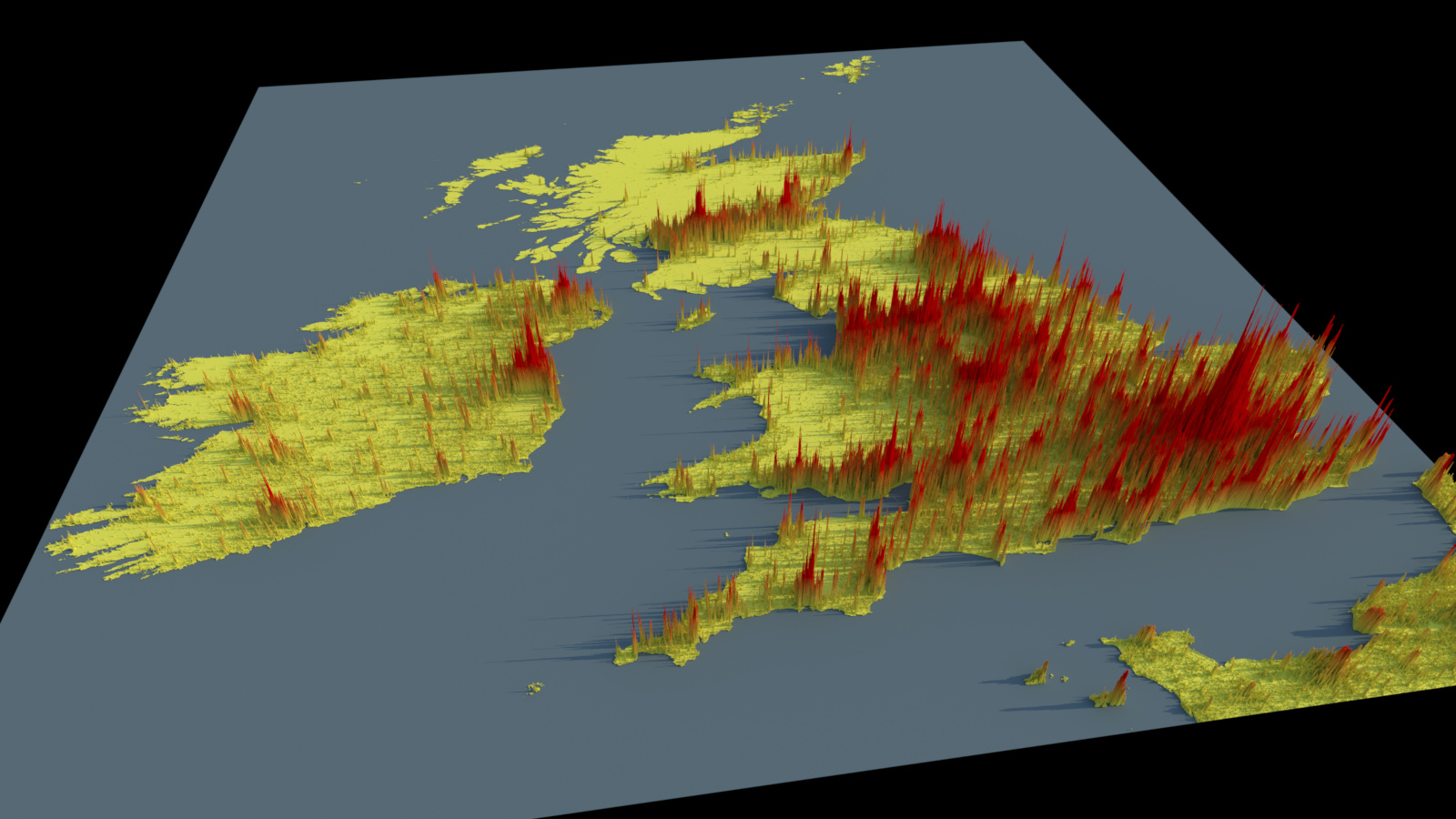
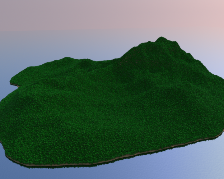
A few weeks ago I noticed on various social media sites some creative and interesting renderings of 3D maps of countries showing their population density as colour-shaded bars extending vertically upwards proportional to the population density values, the original source of which was Alasdair Rae. They’re lit with a fairly low-angled soft light, simulating an early/late sun, which also allows the columns’ shadows to highlight magnitude as well.
I decided I’d try and see what would be required for Imagine to be able to create and render similar looking renders from scratch, using only Imagine and the original source data.
The original data was in GeoTIFF format, which is basically TIFF format but with specific metadata encoding geographic properties like projection and lat/long co-ordinates (which I ignored for the moment), and the data type is normally float32 or float64 (double). Imagine already had support for reading TIFF files in general, but not for reading values as full double-width (float64) floats, so I had to implement support for that.
I then created a Scene Builder plugin (a plugin in Imagine’s UI which can procedurally generate scenes based on input parameters) to generate geometry consisting of small cubes/cuboids based off the data values in the image files, using input image X position for the 3D X axis, input image Y position for the 3D Z axis and the population density values for the Y axis height. Values below a threshold would not generate any geo (i.e. in the ocean with no land).
I also had to merge multiple images together, as each source image represented smaller geographic areas, with boundaries across multiple images for some of the regions I was interested in. For this I wrote custom code as part of the Scene Builder plugin UI to do manual single file / batch merging based off index coordinates.
Functionality to then shade the materials (height falloff gradient, mixed with a 3D grid texture), as well as render the image already existed in Imagine, so I was then easily able to render these:
I ended up ‘cheating’ slightly by not creating full voxel representations of stacks of cubes for per cell columns, instead just using single stretched cuboids to save geometry memory.
One issue with these renders is they’re just using the original source data projection in image space mapped to 3D space, which for places far from the equator like the UK, ends up squashing things quite a bit: I’d need to re-project the data in QGIS to rectify that, which maybe I’ll do in the future, as I do think they look pretty nice.
Some of the source data also seems to have artifacts (extra non-existent land-mass based off rasterising the image input data) in coastal areas, so to render these more nicely, Imagine’s unlikely to be the tool to do these image-space data touch-ups.
This is another comparison of C++ compiler benchmarks on Linux using my Imagine renderer as the benchmark, almost three years since I did the last set of benchmarks.
This time, I’m only comparing versions of GCC and Clang, but I am also comparing the -Os optimisation level in addition to -O2 and -O3.
As with the previous benchmarks I did, I’m sticking with just comparing the standard “stock” optimisation levels, as it’s generally the starting point for compiler flags, and it makes things a fair bit easier, rather than trying every single combination of flags different compilers can support.
As it stands now, Imagine consists of 143,682 lines of C++ in 458 implementation files (.cpp), and 68,937 lines of C++ in 579 header files, for a total of 212,619 lines of code.
The compilers that I’m comparing are:
GCC 4.8.5
GCC 4.9.3
GCC 5.4
GCC 6.3
GCC 7.1
Clang 3.8
Clang 3.9
Clang 4.0
Clang 5.0
GCC 4.8.5, GCC 5.4 and Clang 3.8 were Ubuntu packages, the other versions I compiled from source, using the methods recommended in the respective documentation.
The machine the tests were run on is the same machine the previous benchmarks were run on, but it now has an SSD system disk (which I ran the tests on in terms of target compilation), and a more up-to-date Linux distribution (Ubuntu 16.04 LTS). The machine is a dual socket Intel Xeon E5-2643 (3.3 Ghz) of Sandy Bridge vintage. Imagine’s code has also changed quite a bit in key areas, so these tests can’t be directly compared to the previous tests.
This time I didn’t run any microbenchmarks, just three different renders of different things in Imagine, basically rendering three different scenes. Due to the amount of things Imagine will be doing (ray tracing, light transport, material evaluation, splatting, etc, etc) this does mean that there’s a fair chance that code generated for different aspects can’t really be identified, as the timing will be for the render as a whole, but I think it still provides some indication as to what the compilers are doing relative to each other.
First of all I compared compilation time of all the compilers, building all of Imagine using different numbers of jobs (threads), from 16 (the total number of logical cores / threads my machine supports), down to 2. This was to try and isolate how parallel compilation can be (in particular with hyperthreading) when disk IO is a factor. Imagine’s source code was on an SSD, as was the directory for compiling.
Three runs from clean were done with each combination, and the time was timed with the command line ‘time’ command in front of the ‘make -jx’ command.
The graph below shows the results (mean averages).
As can be seen, there’s a fairly obvious pattern of O3 builds taking slightly longer than O2 builds, and Os builds taking slightly less than O2 builds as one would expect. In GCC, going from 8 to 16 threads (so effectively using hyperthreading on the machine, although it’s not clear what the scheduler was doing) gave practically no benefit in the older GCC versions, with a possible tiny benefit with 6.3 and 7.1, although 6.3 and 7.1 take noticeably longer to compile than older versions.
Thread scalability after that is relatively close to linear, the difference probably being link time which cannot be parallelised as much.
Clang is consistently slower than GCC to build. I saw this in my previous tests I ran almost three years ago, and while in those tests I incorrectly enabled asserts when building it from source, making Clang builds slightly slower, even when disabling asserts back then it was still slower than GCC. This time I made sure asserts weren’t enabled, and it still seems to be slower than GCC, which seems to be against conventional wisdom, however it seems pretty consistent here. 5/6 years ago, I definitely found Clang faster to compile than GCC (4.2/4.4) when I benchmarked it, but that no longer seems to be the case.
Executable Size:
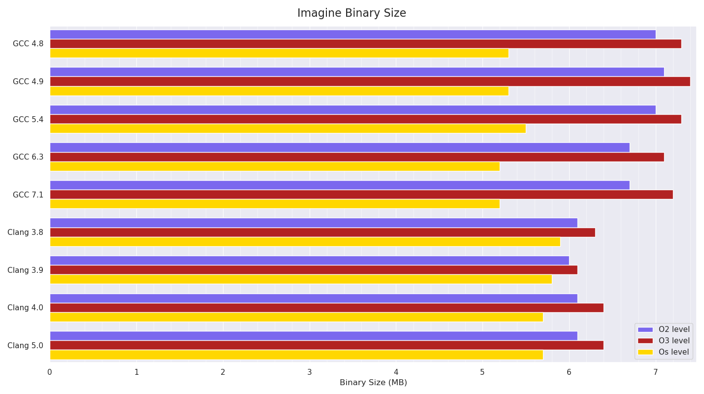
Below is a graph of the resultant executable size:
The pattern of O3 builds being bigger than O2 builds due to more aggressive optimisations (probably mainly more inlining and loop unrolling) is visible, and it’s noticeable how much smaller than O2 builds GCC’s Os builds are compared to Clang’s.
Rendering benchmarks
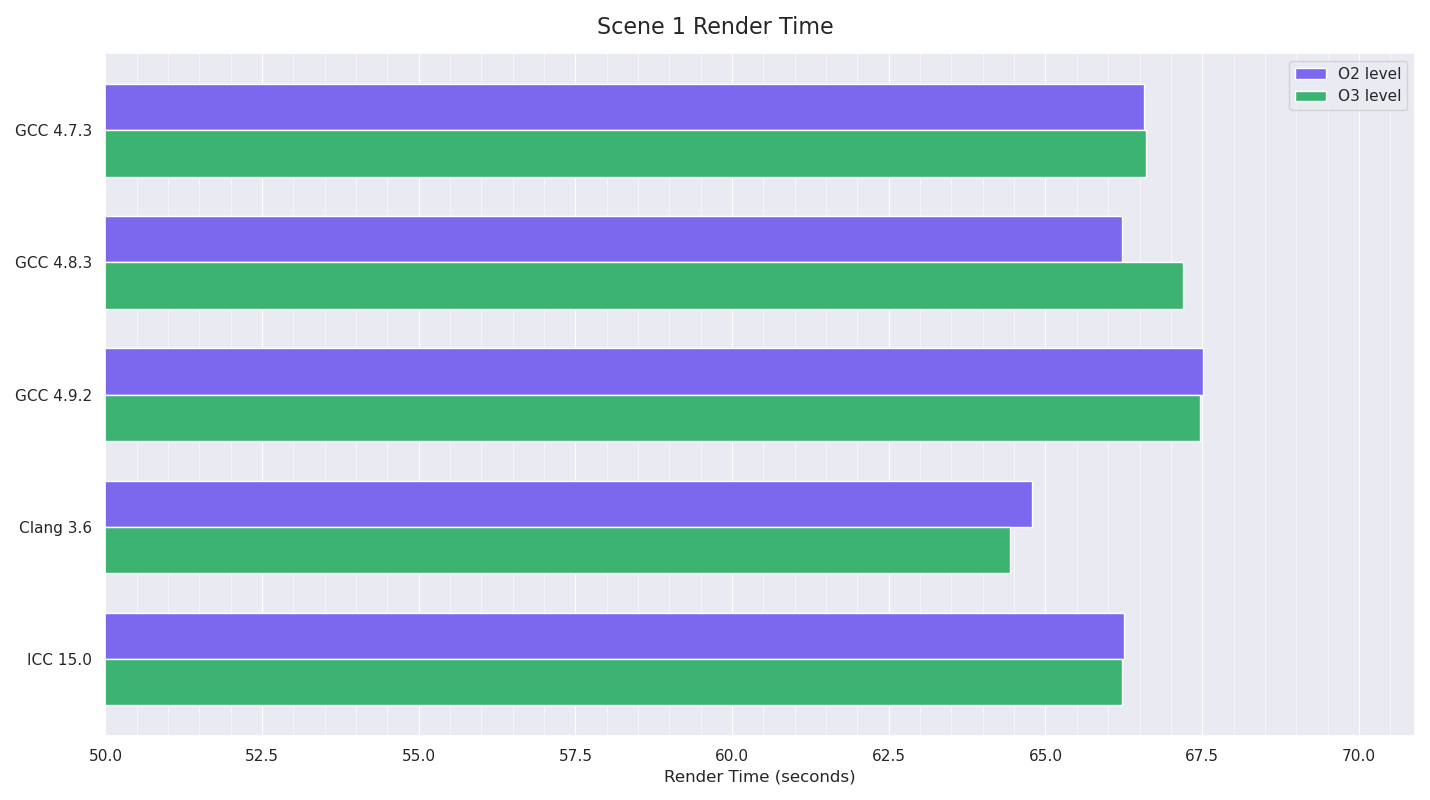
Scene 1:
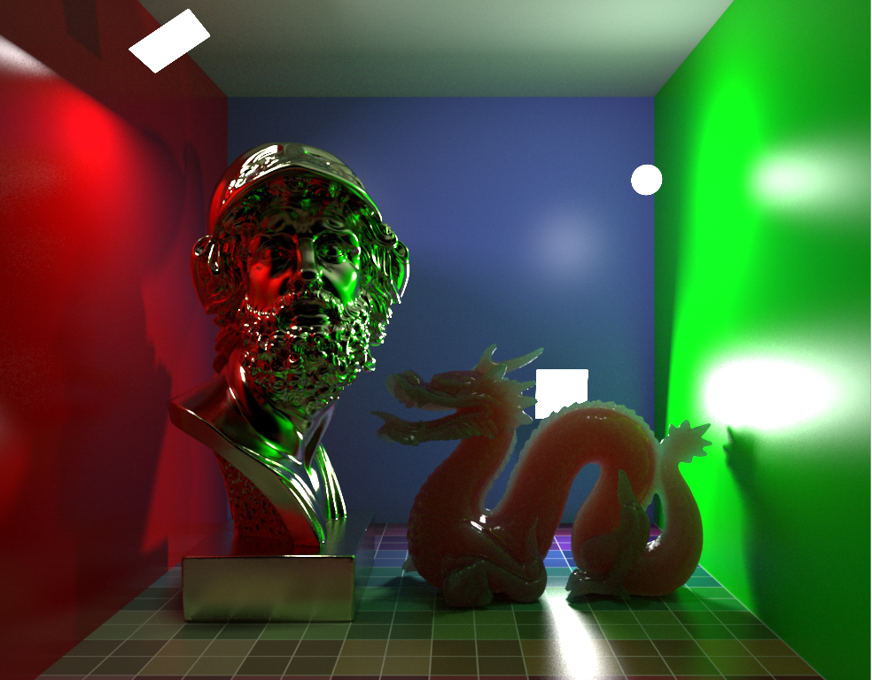
Scene 1 consisted of a Cornell box (floor diffuse procedural texture with Beckmann microfacet spec lobe, walls diffuse + Beckmann microfacet spec lobes), with one bust model consisting of 544k triangles with a conductor microfacet BSDF (GGX), a dragon model consisting of 535k triangles with dielectric refractive lobe with brute force internal scattering for SSS with multiple scattering, and Beckmann microfacet dielectric lobe.
Three area lights (two quads, one sphere) were in the scene, each of which was sampled per hit / scatter (for next event estimation).
The resolution was 1024x768, with max path length of 6, using a volumetric integrator (which calculates full transmission for shadows, so it can’t early out in most cases), in non-progressive mode, using 144 stratified samples per pixel in basic pathtracing mode (no splitting) with MIS. The Mitchell-Netravali pixel filter was used for splatting.
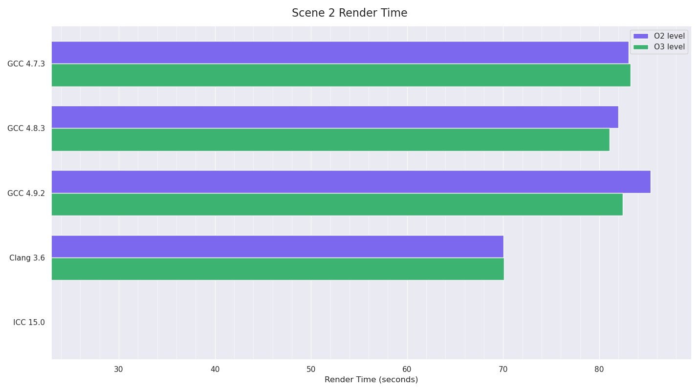
Scene 2:
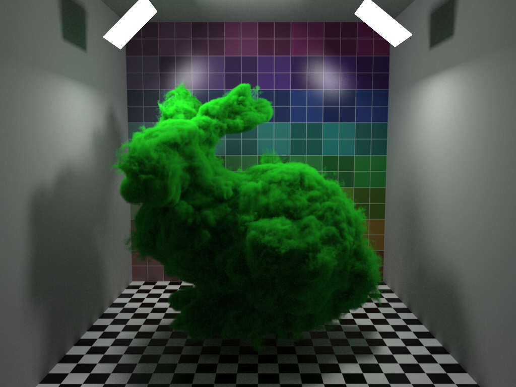
Scene 2 again consisted of a Cornell box, but with more basic materials (only the back wall had a spec lobe on in addition to diffuse), with two quad area lights, and a dense voxel grid volumetric bunny (converted from OpenVDB examples) with an Isotropic phase function. The resolution was again 1024x768, with max path length of 6, with 81 stratified samples used in non-progressive mode.
The volumetric integrator was used, with Woodcock tracking volume sampling for the heterogenous voxel volume, with multiple scattering, and two transmittance samples per volume scatter event per light sample. Both lights were sampled per surface and volume scatter event for next event estimation. Volume roughening (falling back to nearest neighbour voxel lookup after ray roughness / throughput reaches a threshold) was turned off, so full trilinear voxel lookups were always done.
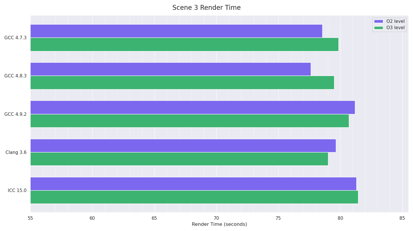
Scene 3:
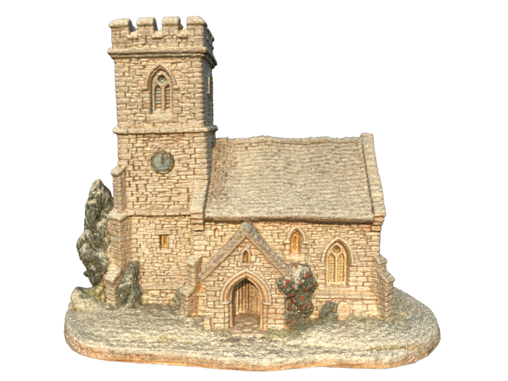
Scene 3 consisted of a single 10M triangle mesh of a scanned church ornament, with a diffuse texture provided by a 1M point pointcloud lookup texture (KDTree).
A very large filter radius was needed on the point lookups, due to the weird arrangements of the colour point values in the pointcloud in order to not have gaps in the resulting texture. A constant Beckmann spec lobe was also on the material.
A single Physical Sky Environment light was in the scene, with Environment Directional culling (culling directions on the Environment light that aren’t actually visible from the surface normal) disabled.
The resolution was 1024x768, max path length was 5, and a non-volumetric integrator was used this time, meaning occlusion ray traversal could early-out instead of having to find the closest hit and test transmittance through materials as the volume tests above had to. 81 stratified samples per pixel were used in non-progressive mode, with MIS path tracing.
Performance Results
Six runs of each were done, restarting each time to account for possible different memory layouts - Imagine is NUMA aware where possible, trying very hard to allocate and write (first touch) memory dedicated to the core/socket that will be running, but some things like triangles / geometry / acceleration structures can’t really be made NUMA-aware without duplicating memory which doesn’t really make sense, so it’s somewhat down to luck where memory will be (in terms of attached to which socket). 16 threads were used for rendering, and render thread affinity was set. The times are in seconds, and are for pure rendering (no loading, scene building or acceleration structure building included in the times), and were measured with code within Imagine.
Mean averages are graphed below.
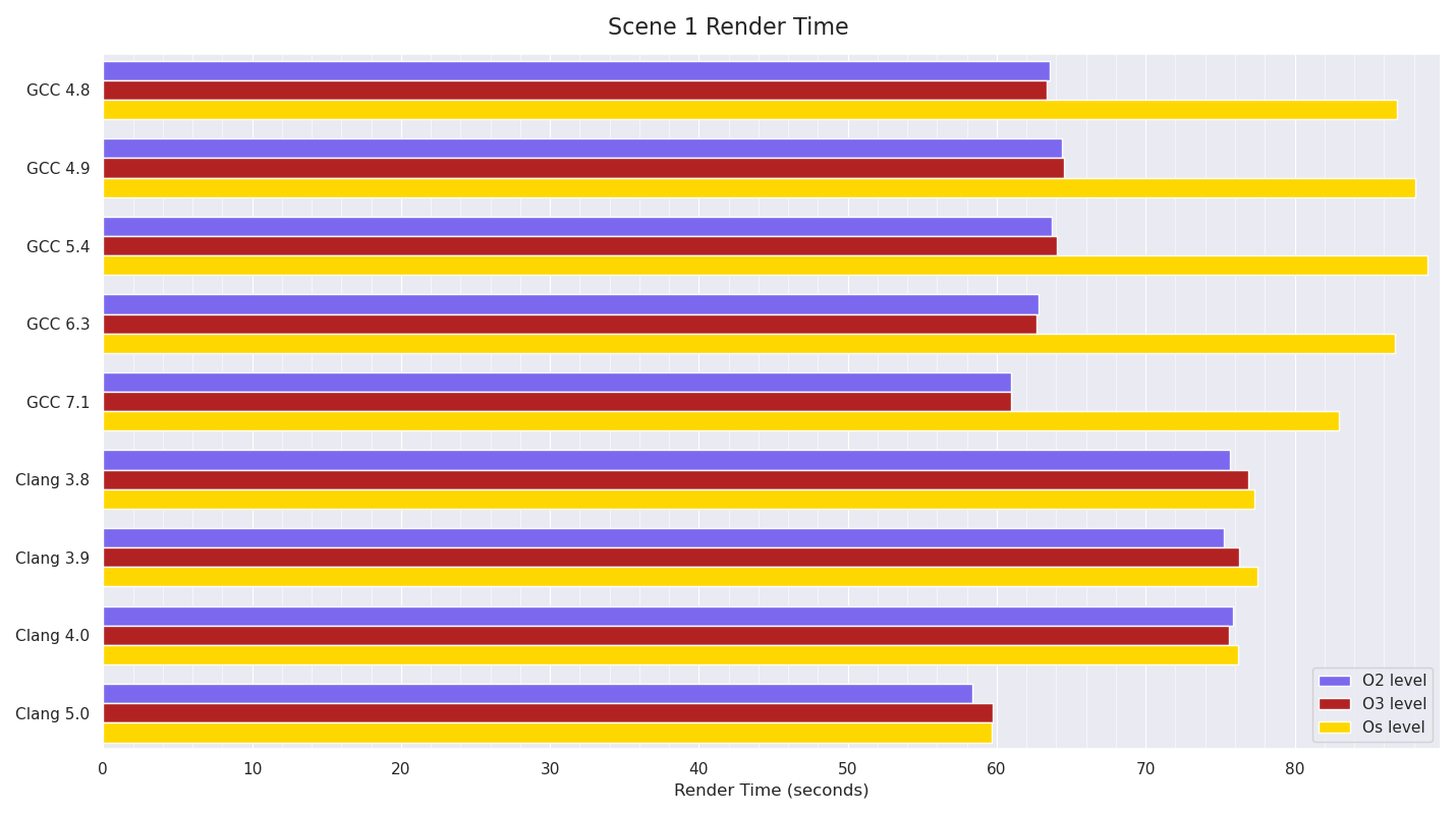
Scene 1
Scene 1 results show GCC 7.1 made some improvements over previous GCC versions, and that GCC’s Os builds are noticeably slower than its O2 or O3 ones. Until Clang 5.0, Clang was noticeably slower than GCC, however Clang 5.0 managed to just beat GCC 7.1’s numbers. Interestingly, Clang’s Os numbers show almost no difference to its more optimised builds, in contrast to GCC’s ratio between the optimisation levels.
Scene 2
Scene 2 shows a regression in performance going from GCC 4.9 to 5.4, which still hasn’t been recovered in GCC 7.1. Clang wins these by a comfortable margin.
Again, Clang’s consistency between different optimisation levels is very close, in contrast to GCC’s, which is more pronounced.
Scene 3
Scene 3 is fairly similar to Scene 1 in that GCC 7.1 makes slight gains over previous GCC versions (and is the fastest), while until Clang 5.0, Clang was noticeably slower than GCC. Clang 5.0 almost makes up the gap to GCC 7.1.
Conclusion
Given these benchmarks are pretty much “overall” benchmarks, given within each test Imagine is doing so many different things, it’s very likely things are averaging out between the compilers,
however, it does seem that Clang 5.0 made significant improvements over Clang 4.0 in two of the tests, becoming the new fastest in Scene 1 and almost matching GCC 7.1 in Scene 3. GCC 7.1 is the fastest in Scene 3, and almost the fastest in Scene 1, but GCC’s speed regression from 4.9 -> 5.4 in Scene 2 still impacts GCC 7.1, meaning Clang completely dominated Scene 2.
What was very interesting to me was the speed penalty GCC’s Os builds have compared to Clang’s Os builds. Given the executable size graph shows a similar ratio in terms of GCC’s Os builds being noticeably smaller than GCC’s O2 builds than Clang’s Os builds are than Clang’s O2 builds, it seems fairly obvious from the executable sizes produced that Clang is still fairly aggressively optimising Os builds, in contrast to GCC which seems to much more strongly prioritise smaller executable size.
Over the past year I’ve been working on (and to a much greater extent optimising) an image texture cache system for Imagine.
Imagine has had some form of reading planar (entire) images since very early on, but other than a slightly hacky integration of OpenImageIO (but that did work efficiently) into Imagine just to test things, it hasn’t had proper integrated support for reading (and more importantly paging) partial images lazily on-demand. This ability is essential for a production level renderer in VFX, as the size and number of image textures used in VFX for rendering is pretty extreme.
I could have just integrated OpenImageIO properly into Imagine, but there were a few reasons I didn’t want to do this: First and foremost, I wanted to write my own and experiment with different ways of handling concurrency, scalability as well as eviction. Second, I already had my own file readers / writers and didn’t like some of OIIO’s dependencies. Further reasons were that OIIO comes with a fair bit of baggage which at least in my use-case for texture reading, I didn’t care that much about: in particular rather bloated data structures in some cases (partly due to Field3D support requiring matrices). It also had some limitations: didn’t support constant tiles, although in fairness there aren’t any open file formats that support this, although I’d like to investigate creating a file format at some point - which can make a huge difference in terms of File I/O bandwidth (which is a very important bottleneck for high-end VFX rendering), it doesn’t natively support texture atlassing (e.g. UDIMs) and I was also not completely convinced by its efficiency or scalability, although it definitely is a capable and production-proven library. I also wanted to experiment with adding new features like on-the-fly compression of tile data, and doing this in a clean and minimal code-base would be much easier.
Imagine already had file readers, but they only supported reading planar images into image buffer classes, so the first step was to provide the ability for a file reader to describe the metadata of an image file, and fill in the details, including resolution, number of channels, data type and mipmap levels.
In terms of general storage of image textures, I created something that’s essentially similar to OpenImageIO’s overall design, whereby there are two main items stored in the cache: image items, which represent the actual image file metadata, and image tiles, which represent the pixel data of the images themselves, broken into small tiles. However I wanted to try slightly different algorithms to what OpenImageIO uses for tile eviction, as I had the suspicion the method it uses (mark and sweep iterator over entire tile cache) wasn’t the best approach from a speed and scalability perspective. One of the ideas I had in mind was not actually removing any tile items at all at eviction time, but only freeing the pixel data itself. This would use more overall infrastructure memory (excluding pixel data), but it should reduce the need to lock the entire tile cache very slightly, which hopefully would help scalability and performance. Given that classes and structs representing texture items and texture tiles would never be freed at tile eviction for paging, it was therefore extremely important that they be as memory efficient as possible.
I made a conscious decision to not separate different channel images based on tiles requested based on the channels requested - that is, if an RGBA image was loaded, but only the A channel was requested, I’d still load all four channels into memory instead of partitioning each tile and having an extra dimension to have to cope with for the tile hashes. This was partly to keep things simpler, but also to constrain the number of tiles given I wanted to not have to free the tile items at all when paging, only freeing the pixel data. It would mean however, that in certain situations like the example given above, memory usage would be higher than needed. However, as is generally done in high-end VFX, the solution here is to make sure each texture image just contains one set of channels, so the above example would have two textures, one for the RGB channels and a separate one for the A channel.
I also made a decision to not use lazy texture loading for HDRI environment maps, but to keep those separate, partly because you’re effectively point-sampling them anyway (definitely at construction time to build the CDFs), but also to keep texture requests down for this type of illumination.
I also wanted to be able to categorise images based on purpose, both for allowing different caching / eviction strategies for different types and to allow different types of filtering to be done on them: there are some situations like for alpha/presence maps and layering mask/mix maps that it’s generally better to err on the side of less filtering, even at the expense of possible aliasing.
To begin with I started with just the bare basics as I wanted to investigate and experiment with different ways of doing things to see the effects they would have. As a starting point I initially just had a single mutex around each map collection, so that I could see what the extreme worst-case scenario was.
Imagine was using ray differentials to calculate texture filter regions and thus the mipmap levels to pull in of the textures, and doing trilinear filtering to combine mipmap levels.
Tests even with just a single plane polygon in the scene with one texture were as expected pretty abysmal, with CPU utilisation on a 16 core / 2 socket system hovering around 300% (instead of the ideal of 1600%).
I implemented per-thread microcaches that stored LRU arrays of pairs of both the texture items and their hashes and tile items and their hashes, which was used to lookup textures before going to the main cache and in this contrived scenario, other than for the first few buckets where all threads were initially opening file and reading images, CPU utilisation went up to the expected 1600%, fully utilising the available cores.
Testing with other simple objects added to the scene with the same texture (so that there were now indirect rays being fired in an incoherent fashion) could scale to a degree if I increased the microcache sizes, but this wasn’t going to be a good approach, as the single mutexes around the individual map containers were clearly the bottleneck.
So I needed to come up with a solution which would scale well with many threads. In the end I settled on writing my own map container wrapper similar to Java’s ConcurrentHashMap (which is also similar to what OIIO uses, and how Linux’s hashed spinlocks work), which splits the map into different “bins” (although I called my version “shards” which is more in mapping to the database partitioning technique). Each “shard” contains its own isolated map and mutex, and the shard to use for lookup and inserting values is chosen by using the modulus of the hash value for the key, based on the number of shards. It’s then possible to lock just this shard and lookup within its individual map to find / set the value as required, while other concurrent requests from other threads will have no contention, so long as they map to different shards. If they do map to the same shard, then there will be a certain amount of contention. So it’s extremely important to have a very good hash function which distributes well over the domain space. In my case, after an awful lot of trial and error and playing around with the avalanche effect of hashes for tiles, I came up with hashes which seem to work quite well: I used Austin Appleby’s MurmurHash3 for hashing the filename, generating a 32-bit integer, which allows lookups of the texture item itself.
For tile items, I ended up using a 64-bit integer of the 32-bit texture item hash shifted 32-bits to the left, being added to by the mipmap level shifted 24-bits to the left, then the tileY coordinate shifted 14-bits to the left with the final tileX coordinate unshifted.
Another very important factor which was important is mixing the hash used to lookup the shard so that it doesn’t have the same correlation within the shard’s hash map, which can severely affect the efficiency and load factor of hash maps within each shard.
With this implementation, scaleability was perfect on 16 threads with these simple scenes, so I then attempted to stress-test it with more complex test scenes and finally as close to a production level scene as I could fabricate texture-wise.
I tested initial scalability of the locking by using “virtual” image texture readers which just generated texture colours procedurally (tiled based) so as not to be limited by disk speed or OS-level disk caching.
Tests with the extreme worse case scenario (just a single mutex around the containers - and using the less-than-ideal std::map<> to begin with for lookup structures) were understandably atrociously bad, although interestingly scaling on Linux was much better than on OS X, probably due to Linux’s Futexes.
Scalability with sharded maps was much better on OS X, and noticeably better on Linux, scaling close to linearly with 32 shards for both maps. Changing the underlying map type to std::unordered_map (hashmap) reduced lookup time by around 25%, which was not as much as I had hoped. I experimented with setting the initial bucket count and max load factor for the maps and this reduced lookup time by around 10% again, and at this point I was slightly worried that my hashes weren’t as well distributed as I thought - so I thought this would be a good time to both check the distribution of the hashmaps and see if the strategy of not deleting items from the maps gave any benefit. Without controlling the load factor and initial bucket count, once paging started happening, not deleting items seemed to give a slight speedup - possibly due to the fact tombstones didn’t need to be used to mark items as deleted. However when optimising the initial load factor and bucket count, the difference was negligible - probably due to hashes mapping very nicely to open buckets with very few collisions happening. However the ability to not delete tile items did mean that in the texture stats I was able to very accurately track unique texture data read during paging, which is quite useful, and I kept this as an option.
I experimented at this point with increasing the microcache sizes a bit (to 16 entries per thread for both), and for simple scenes with less than 60 textures this made a noticeable difference (especially with paging enabled, as it meant if an item was in a microcache it was recently used so it shouldn’t be evicted), but once each ray hit was evaluating more than 10 textures for layered materials, these microcaches became barely useful due to almost random thrashing between vertices per path. I have some ideas for trying to use more tree-like data structures for them in order to take advantage of ray-tree coherence, but the best approach here would just be full-on deferred ray batching / sorting, so I’m not convinced it’s going to be worth it.
At this point without having to page textures to fit in a particular memory limit, my texture cache was faster than OpenImageIO for pretty much identical numbers of texture evaluations, but with aggressive paging turned on OpenImageIO was noticeably faster. Looking at the stats between the two, it was obvious that my naive eviction method was causing an awful lot of duplicate reads (still using virtual file readers, so no disk access was taking place, only memory allocations and procedural textures). I decided to just copy OpenImageIO’s clever method of marking a tile as recently used with an atomic variable, allowing a very cheap compare-and-swap to be done, allowing skipping recently-used tiles very accurately and efficiently, although with a slightly less cumbersome mark-and-sweep process. This change made a huge amount of difference, with my texture cache now being ~5-10% faster than OpenImageIO. I also experimented with over-evicting based on a ratio to prevent continual locking: if a request for a new image needed 2KB of data, I’d actually free more than that, so as to do more work within the one lock event meaning it would be more likely the next request for a new texture would not need to lock as well to evict - this made a noticeable improvement (after experimentation I settled on doubling the target eviction size).
I then decided to move to proper tiled based image textures, testing both TIFF (briefly) and OpenEXR. I noticed immediately with OpenEXR that using the worker thread calling OpenEXR to read images (i.e. with the threadpool size set to 0) had severe contention issues, caused by redundant locking in IlmBase’s ThreadPool class. Larry Gritz had also spotted this issue previously and had a fix for it on GitHub which allowed EXR reading with worker threads to scale a lot better. Along the way of testing with bigger and bigger scenes I had to fix several issues with ray differentials not propagating correctly causing incorrect point-sampling of the lowest level mipmaps, which obviously slows things down to a halt. In the end for some edge cases I had to build in texture filtering based on approximate ray-width as a backup for when ray differentials failed (due to incorrect/inconsistent UVs or missing UVs on meshes).
I then decided to scale things up to an extreme test to stress test the cache: I tested with a large cornell-box style scene containing four production-scale hero objects - many different components with different materials, all with UDIMed textures with varying numbers of layers (one to three, controlled with mask textures controlling mixes), with diffuse, specular colour, specular roughness, clearcoat reflection and bump textures being utilised for most (but not all) materials. The floor and the walls of the Cornell box also had diffuse textures of 10x10 tiles of UDIMs (so each plane other than the ceiling consisted of 100 texture files).
The total number of image texture files was 898, and I made use of OpenEXR format tiled mipmaps of 16-bit half format at 8K, the tile size being 32x32. Total size on disk for all textures was over 320 GB.
I tested with path length set to 6, so there would be a large amount of incoherent texture accesses.
Testing this scene showed it worked very well, and was consistently slightly faster than OIIO - this is probably partly due to less locking that I do in general, but probably also because my texture cache has full integrated support for UDIMs, so can batch up requests to adjacent tiles on UDIM borders and when filtering to reduce locking even more.
I experimented with adding support for compressing pixel tile data in memory using LZ4 - the idea being that for constant tiles (which no open standard tiled file format supports at present, so there’s no way to detect them up front) it might be a way to detect these on-the-fly with a tiny bit of overhead. Testing with simple textures worked well, and if the compression ratio was excellent it was obvious it was a constant tile, and I could mark it as such and not bother evicting it, which brought a slight speed-up. If the compression ratio was just good, there was some constant data in the tile, and it meant I could fit more in memory without going back to disk when paging. However, with real-world textures painted in Mari it didn’t work as well, as outside the UV’d area Mari tends to distort texture detail instead of leaving it black, so there’s still texture detail there taking up space. One situation where compressing did still provide benefits with real-world textures was with layer masks texture maps used for mixing / isolation, which are generally less detailed anyway - it was possible to often detect constant tiles and even if there weren’t entire constant tiles still compress image data usefully within tiles.
So I now have a very fast, efficient and scalable image texture cache - I still think there could be better texture formats than OpenEXR which unfortunately has become the standard for textures at VFX level but is seemingly somewhat abandoned: OpenEXR’s threading is really bad, and the use of threadpools doesn’t really make sense for reading multiple random tiles per random mipmap level in parallel in a path tracer - it’s possible with coherent access using threadpools is still a win for rendering (it definitely does make sense to use threadpools to speed up reading a single large entire image for use in image viewers and compositors, and for writing images), but I think it makes sense that a file format for rendering be completely stateless, with metadata decoded once, and then any number of threads be able to read/uncompress at will without dependencies / state controls - obviously depending on how the image is compressed there may be problems here, but a balance needs to be found. In addition OpenEXR doesn’t support 8-bit or 16-bit integer formats which can be very efficient for certain types of data (masks / isolation maps), neither does it support constant tiles or instanced tiles. So I’m tempted to try creating a texture format just for rendering, optimised for extremely fast random access.
I’ve just finished implementing the first pass of the ability to record events that happen during light transport, and visualise them in Imagine’s OpenGL viewer. I’d been having issues with light sampling issues with complex light setups with many lights, and just looking at the code and debugging what was going on from within gdb wasn’t really getting me anywhere.
So I decided that as Imagine has a GUI (in non-embedded mode, anyway), it would be fairly easy to record events like path vertices, light sample positions, etc, during light transport and then later display them in the viewer. I ended up creating a separate DebugRenderer integrator for this, which I’m not completely happy with as it means code duplication in order to replicate light transport and light sampling, but integrating this event recording (at a fine grained level) brought with it some time overheads - definitely when recording events, as expected, but it was also even slightly noticeable when it was turned off in the light sampling code, presumably due to extra branching - but more importantly it complicated the existing code quite a bit, so for the moment I’m going to keep it like this.
It’s allowed me to very easily identify issues with spherical analytical light sampling in Imagine, as well identifying some other light sampling issues, and with some future improvements to support volume scattering events as well as better view-time filtering (to allow constraining the preview of these events to useful subsections), it should be better still.
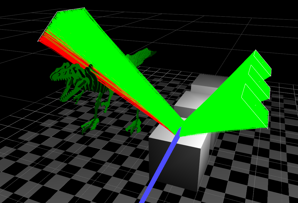
The below images show the rendered scene and the visualisation of a sub-set of rays hitting the top of a cube for the first hit event from the camera: blue lines are camera rays, green lines are successful next event estimation rays which found a light and red lines show next event estimation rays which were occluded.
It can also show un-sample-able light samples (back-facing), secondary bounce rays (tagged/coloured diffuse, glossy or specular) and exit rays which didn’t hit anything in the scene.
I’ve now implemented pretty robust support for statistics in Imagine, both count-based (counters of events) and time-based: having statistics is important in order to know how to optimise your scene and work out where time is being spent from a user’s point-of-view. Imagine has three modes statistics can be set to: Off, Lightweight and Full.
Off and Lightweight under-the-hood are the same (although Off doesn’t print to console/write to file the results) and just increments counters of events, like rays fired by type, maximum path length, BSDF evaluations, texture reads, etc. This mode has no measurable overhead (I couldn’t see the difference in a 1 hour render, anyway), although technically the code is doing a few more integer additions. At first I tried using global atomic counters, but these did have a slight overhead (atomic variables can still have contention issues), so in the end I made use of per-render-thread statistics which got added together at the end of the render.
Full adds time-based counting to the mix, unfortunately with a slight overhead (~1-3% of total render time depending on how many timers I used and where) as accurately timing lots of events in a fine-grained manner has a small but noticeable overhead, but in a (not-quite-yet in Imagine’s case) production-level renderer, time statistics can be immensely useful (as long as they’re accurate) in identifying bottlenecks / inefficiencies in rendering scenes. The stats aren’t quite as comprehensive as PRMan’s, but they’re more comprehensive than any other commercial renderer I’ve used.
I also added heatmap output support from a render bucket point-of-view, which is just the total time each render bucket took normalised over the entire image which quickly shows you where the majority of the time was spent (see below for an example, where hair rendering takes up the bulk of the time) and a slightly-hacky per-pixel CPU time AOV output.
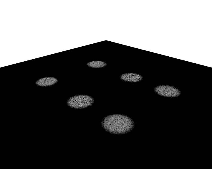
I’ve also been working on “localised” light sampling, where instead of randomly picking lights to sample either uniformly or from a distribution based off a light’s constant total emission, you “localise” the picking of lights to the shading point(s) being shaded/lit - the aim being to ensure you sample lights that will give a greater contribution than lights far away, which can make a tremendous difference when there are thousands of lights in a scene. In Imagine’s case, I’ve done this based on the direction and distance (with a bit extra for spot lights), and implemented a double-stage lookup, where when ray intersections need to be lit by direct lighting, I build up a small (up to 128) per-thread distribution based off approximate radiance of random lights. This then allows discarding of lights which don’t actually contribute any lighting to that particular intersection point. Care has to be taken to balance the distribution pick PDF to ensure lighting doesn’t get biased by this.
While this is more work and therefore more expensive, in that there’s much greater chance that lights being picked are going to contribute lighting to shading points (it doesn’t test occlusion visibility though, so there’s still a chance that the light might be blocked by something), it can reduce noise considerably as the below contrived scene with six spot lights shows. Four samples per-pixel were used, each picking one random light in the first case. Once complex geometry mesh lights (i.e. self-shadowing/occluding) and environment lights come into the picture and there are mixed light types in the scene it doesn’t work as well, but it still gives a huge improvement in certain scenes.
I’ve also added checkpoint support (resuming renders), by saving the sample count per-pixel to the output EXR which can then be read in again and resumed, along with a bit of metadata.
I’ve also reduced memory usage a bit more and started work on PrimVar support.
Recently, I had been about to upgrade my Linux distro on my main workstation at home, and this brought an upgrade to GCC 4.8 from 4.7 as the base GCC version. Before I upgraded the distro I tried building Imagine with 4.8.3 built from source, and needed to fix some template code as g++ 4.8+ (ICC has never liked it either) now doesn’t like using pure abstract classes as a template type. I made this change to the code, and did some quick approximate benchmarks between 4.7.3 and 4.8.3 which showed there wasn’t really any improvement, so I decided to try 4.9.2 which had just been released. This seemed to showed a fairly serious regression in terms of speed (speed being a pretty important aspect for a renderer), so I decided I’d do a more comprehensive comparison of the latest main compilers for the Linux platform, as back in 2011 and 2012 I used to do compiler benchmarks (GCC, Clang and ICC) regularly every six months or so on my own code (including Imagine), and on the commercial VFX compositor made by the company I worked for at the time, and it had been a while since I’d compared them myself.
I’ve never really liked just doing micro-benchmarks/synthetic benchmarks of just loops, etc of simple code, as they can paint a distorted picture of what’s going on, which can’t always be realised when the same code is put in context within other code - a good example of this is C++ virtual function overhead, which I’ve previously benchmarked, and while it’s possible to see overheads in micro-benchmarks, the same code within an actual real application shows no issues (at least in my particular usage of them) - so I always try to benchmark code doing what it was designed for from a user’s perspective: in Imagine’s case, this is rendering, or aspects related to that.
As it stands now, Imagine consists of over 164,000 lines of C++ code (including comments) in 386 .cpp files and 484 .h files, included heavily (more-so than I’d like, as it causes pretty severe final binary code bloat) templated code for everything from the acceleration structures, image texture / filtering infrastructure to geometry attribute / indices / triangle type code and a fair amount of SSE intrinsics usage for some of the acceleration structures, image filtering, procedural noise textures and triangle packet intersection code. The rest of the code is standard 2003 C++ - GCC 4.1.2 is still used heavily in the VFX industry (due to plugin ABI compatibility issues), so I still want to be able to build Imagine with this compiler if need be. Other than (optional) image library libs (OpenEXR, libpng, libtiff, libjpeg) for file readers/writers, there are no other requirements/dependencies Imagine needs to build.
The compilers I eventually benchmarked were: GCC 4.7.3, GCC 4.8.3, GCC 4.9.2, Clang 3.6 (prerelease from SVN - with -enable-optimized configure option) and Intel ICC 15.0 trial. I did spend several hours trying to get GCC 5.0 prerelease built from SVN, but gave up after I couldn’t get it to accept either my system zlib installation or a custom one I built from source - googling seemed to indicate this was a multilib compatibility issue and I could get around it by symlinking include and lib directories for various things, but doing that didn’t work for me. I also wanted to compare earlier GCC versions, but couldn’t get 4.6 or 4.4 to build from source on my system either - again, seemingly due to multilib issues.
Comparing compilers fairly is a difficult thing to do as they all have different abilities in terms of optimisations, and even for the built-in standard -O1/-O2/-O3 optimisation types, they do different things for these. However, given the huge amount of different options they have controlling things like inlining aggressiveness and limits, loop unrolling, vectorisation, etc, it would be vastly time consuming to try every compiler option progressively to try and find the best combination for that version of compiler, although that would be the fairest test in terms of benchmarking the fastest code a particular compiler can produce for a specific set of limitations (instruction support, etc). For this reason, I’m going to stick to just comparing each compiler with both -O2 and -O3 with SSE4 support, as these are generally the starting points for using the compiler.
I decided to run three different rendering tests, each one testing slightly different features of Imagine, although there would obviously be a lot of overlap between the tests, and then two synthetic tests: one of image mipmap creation and the other of procedural noise evaluation.
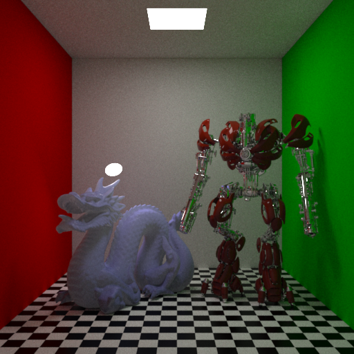
Scene 1 was a fully-enclosed cubic room, but with the front wall plane invisible to camera rays allowing them into the scene. Inside were the Stanford dragon at 1M triangles with a translucent SSS material, and the Katana robot example model with a combination of metal and car paint materials. Two area lights illuminated the scene, a standard ceiling quad and a disc light behind the dragon. This test made use of brute-force multiple-scattering volumetric integration for the SSS, with uni-directional path tracing with MIS, with two light samples taken per direct lighting evaluation. A total of 5 ray bounces were allowed, with a limit for diffuse and glossy of 4, and 5 for reflection rays.
Scene 2 consisted of a large plane with a highly anisotropic metal material with a simple toy train model with diffuse, specular and bump textures and Cook-Torrance-style materials.
There was also a volume primitive backed by dense voxel grids for density and temperature with a (pretty poor) blackbody shader for the emission colour based on the temperature. Trilinear interpolation was used to lookup voxel values. The last object was a toy helicopter with metal and plastic materials, with the rotors animated and quaternion interpolation used for motion blur. An HDR environment light was used. Brute-force multiple-scattering was enabled for the volumetric integration.
Scene 3 was an extremely large plane with reflective surface and a procedural bump texture, with an island mesh with 165,000 instanced trees on it. The trees had diffuse textures on the trunks as well as procedural bump textures (simplex noise), and the leaves were constant diffuse+backlit+CookTorrance spec, with an alpha texture for cut-outs (using stochastic presence sampling for all ray types). An HDR environment light was used. This was rendered as a Deep Image (alpha), so the integrator needed to do extra work collating and possibly merging each pixel sample for each pixel.
I configured Imagine to use completely deterministic sampling (the random numbers used to generate samples were consistent between runs per thread), and all textures were pre-loaded in memory before starting the renders. Similarly geometry processing and acceleration structure building was done before starting the timers, meaning these rendering tests should be completely deterministic in terms of calculations and would only be memory / CPU bound, essentially testing raytracing intersection, light integration, texture lookups, procedural texture evaluation, etc.
-O<n> -fPIC -fp-model fast -msse4 -no-intel-extensions
(plus some experimental tests I later did with: -O3 -no-prec-div -fp-model fast=2 -xHost -inline-level=2).
My system was a dual-socket Xeon quad (E5-2643), with eight physical cores - 16 threads with hyperthreading (which I made use of for the rendering tests). Linux Kernel version was 3.5.
Timings are mean averages over multiple runs, with the system idle and making sure all CPU core temps were under 45 degC to not bias things by allowing turboboost being used differently between runs.
Results
I did some quick compile timing tests (all using eight jobs only to make sure the build wasn’t IO constrained). Three runs of each from a completely clean build, other than for ICC which kept having FlexLM license errors, so I only had the patience to do two runs for ICC. Mean averages are shown.
To my surprise, Clang was slowest: generally I’d previously found that Clang was much faster at compile time than the other compilers, and other recent benchmarks seem to show that picture as well. Running single-threaded builds of Clang and GCC 4.7 showed similar results: 6 minutes 18 secs and 4 minutes 49 seconds respectively, so I’m not sure what happened here.
(Later Edit: it turned out I had built Clang with asserts enabled, which meant it was doing extra work, and meant the timing numbers for Clang for compile times using it were inaccurate, but all other results here are valid from the build).
For the three render scene tests, Imagine was started, pre-renders were done, I ensured all the CPU core temps were under 45 degC and the system was idle, and then I rendered the scene. Rendering was done with 16 threads (using full hyperthreading of the machine), and each thread had its affinity tied to a unique CPU id (using pthread_setaffinity_np()), hopefully meaning there was less scope for the scheduler to bounce threads around different cores leading to cache misses (in the past I’ve noticed more than measurable speed improvements by doing this especially when the machine has multiple CPU sockets). Timing for just the rendering stage was printed to the console. I ran each test separately, restarting Imagine and doing the pre-renders each time (meaning memory for the images, geometry and acceleration structures would very probably be allocated in different places each time).
I did at least four tests with each compiler / optimisation level combination, often doing more when the variance between the numbers looked odd or too large. I saved the render output of two of each combination for checking later (to ensure they’d rendered the correct thing and to compare final output values).
The tests for Scene 1 had Clang as the winner by a fair margin, with GCC 4.9 very slightly slower than the previous GCC versions. Only in Clang’s case was the O3 build noticeably faster than the O2 one.
The tests for Scene 2 also seemed to have Clang as the clear winner, although I couldn’t run the Intel ICC tests as there were severe issues with the acceleration structure build code which only triggered in this test (code branches were being taken that shouldn’t have been possible). For the moment I’m putting this down to an ICC bug (given past experience with ICC, unfortunately it is pretty buggy) as marking a uint32_t class member variable as volatile “fixed” the issue, but it definitely seemed that ICC was emitting code that would not copy across all the bits of a uint32_t and so was truncating it, leaving some bits uninitialised. This code was only running when motion-blur was being used for an object (the helicopter’s blades in this case) - basically a special type of primitive clipping that works well with motion blur bounds. I added debug code to verify that none of the other compiler builds were doing things wrong in that place, and as I didn’t want to test ICC with this volatile modification which shouldn’t have been needed, I just skipped it.
GCC 4.9’s results however, showed that the timings were pretty inconsistent: ranging from 88.43 seconds to 82.39. I couldn’t find any pattern to this: the system was idle, CPU temp was down before starting, output results for all the different compilers matched almost exactly (the fast math option was enabled for all compilers, meaning the compilers weren’t required to always stick to IEEE float precision, and thus there were minor variations in the results of some of their calculations, but the differences of the final render outputs were extremely minor), until I discovered that doing successive renders with the GCC 4.9 builds with the same pre-render state gave much more consistent results. Given that all the builds were doing almost exactly the same thing (very minor floating point value differences as pointed out above), this pointed to data memory layout differences causing this, possibly even due to memory alignment issues, but more likely due to differing memory layouts of things like acceleration structure nodes, geometry, etc affecting memory pre-fetching or branch prediction in some way due to the code GCC 4.9 was generating. None of the other compilers showed this issue. The only other difference with the GCC 4.9 tests was that I had to set LD_LIBRARY_PATH to point to the GCC 4.9.2 install’s lib64 directory for a newer version of libstdc++.so.6 in order to run these builds. However I don’t think this was the cause of these timing inconsistencies as I tried running some of the other compiler executables with this modified LD_LIBRARY_PATH (and verified using LD_DEBUG=files output that this newer lib was being used), and the other compiler builds I tested still didn’t exhibit this issue.
Scene 3’s tests are a much more mixed bag with no outright winner, although the O2 builds of GCC 4.7 and 4.8 were the quickest. Again, GCC 4.9 showed varying results, and as before, using the same pre-render state and doing consecutive renders gave much more consistent results (which I didn’t include in these results).
Due to the fact these rendering tests were testing quite a lot of different things at once, and I was slightly concerned about the fact that the ICC builds couldn’t run Scene 2’s test, as well as the fact that ICC wasn’t winning any of the tests (when I last benchmarked the compilers over two years ago, ICC was consistently > 25% faster than the other compilers), I decided to turn my attention to more simple synthetic tests.
For the two synthetic tests, I stubbed Imagine infrastructure code into much smaller separate executables, with code just running in the main thread (still with affinity set).
The Mipmap test involved opening 6 8K 16-bit half RGB scanline OpenEXR files from disk, keeping them in memory (at full 32-bit float precision after conversion) and repeatedly generating filtered mipmaps for these images, 11 times each in rotation (so effectively doing 66 mipmap generations).
I only started timing after the images were loaded off disk and converted to 32-bit float format, so the benchmark should be CPU and memory constrained only (quite a few memory allocations).
In this test Clang and ICC lagged GCC significantly, with GCC 4.9’s O2 benchmark strangely slower than the other GCC timings.
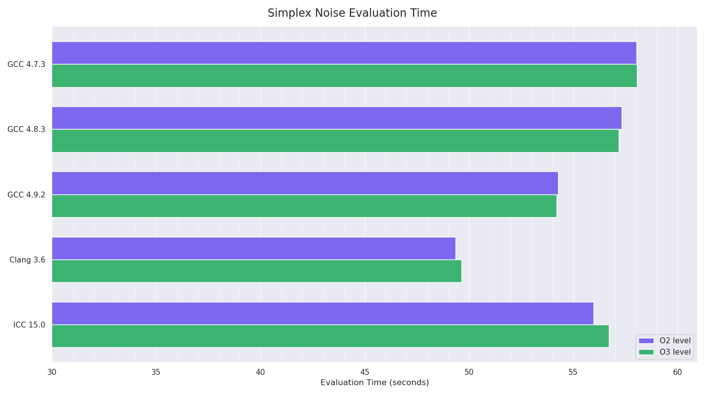
The procedural noise test involved iteratively evaluating 3D simplex noise at regular intervals at positions in the shape of a cube (stepping in each dimension), for a total of 1,194,389,981 evaluations.
I disabled the SSE intrinsics support I had for this code, so it was just pure float / int operations and branching, to see what the compilers could do. This test should be fully CPU-constrained.
Clang won this test by a fair margin, with GCC 4.9 next fastest and ICC followed. I was still really confused by ICC’s poor showing, and started experimenting with more aggressive compiler options: -O3 -no-prec-div -fp-model fast=2 -xHost -inline-level=2
allowing less precision, using all instruction sets the host processor supported and more aggressive inlining at the compiler’s discretion. Doing this knocked a few seconds off the timings for ICC, but I’m almost certain (but didn’t test) doing equivalent things for the other compilers would have done like-wise.
Two years ago, libm’s maths functions (definitely transcendentals like pow(), sin(), etc) were pretty bad in CentOS 4/5 (often to the point that using double precision was significantly faster than the standard float versions), so using ICC meant that it had the ability to replace these functions with Intel’s own optimised ones (which at the time were much faster than libm’s) and statically link them inside the executable. Analysing the symbols in the built executables for ICC and the other compilers showed ICC 15.0 was doing this: most maths symbols for the non-Intel builds were Undefined, with them pointing to GLIBC, whereas ICC’s builds had the symbols in the executable.
So I can only conclude that either GCC and Clang have become much faster over the past couple of years, or libm’s maths functions are a lot faster than they used to be. Both of which I think are probably the case.
I’ll need to do some profiling to work out what’s causing the GCC 4.9 builds to be so inconsistent, as that appears to be why when I first benchmarked with GCC 4.9 it seemed slower.
This isn’t the most comprehensive C++ benchmark, but I think it’s a pretty fair comparison given that the compilers were all limited to a relatively similar degree - while the different compilers do different things at their respective O2/O3 levels, they have the same intent in that they’re recommended starting points, and O3 might be too aggressive in some cases - and taking into account how time-consuming it would be to play around with all the different optimisation flags for the different compilers. I would though have liked to have got GCC 5.0 built from SVN and to also compare the compilers with whole program optimisation, link time optimisation and profile guided optimisation, and to see what benefits those options might have brought over the more standard optimisations.
I ended up spending a fair amount of time on the Katana integration in the end, at least in terms of pulling in geometry attributes and static transforms and exposing materials, so that I could pull production scene geometry into Imagine and see how well it coped against the latest versions of PRMan and Arnold. Initially, before I started work on memory efficiency back in June, it was embarrassingly bad, with Imagine using around 9-11 times as much memory, and Imagine only being able to fit around 52 million unique triangles in 24 GB of RAM. In this original state, Imagine was using gathered vertex attributes, so there was a lot of duplication of data.
The first thing I did was to add the ability to use indexed vertex attributes, and this way the source attributes (points, normals, UVs, etc) could be shared among any triangle / vertex in the mesh, with “just” indices being used to index into them. I put “just” in quotes, because vertex indices can also require a lot of memory, especially if the indices for each attribute are different (i.e. points, normals and UVs all have different indices per vertex).
This change reduced memory usage by around 3 times, but it was still not great. I added logic to detect if certain attributes used the same indices (i.e. normals and UVs), and this allowed me to re-use/share indices for multiple attributes if the indices allowed that. The next thing I experimented with was de-duplication of vertex attributes. In a normal closed mesh consisting of quads, the majority of points, normals and UVs are shared by multiple faces, and annoyingly, DCC tools like Maya don’t seem to put much effort into de-duplicating these attributes (other than points) on export (possibly due to the fact that some renderers like PRMan don’t support specifying indexed attributes explicitly at ingestion stage), so UVs and smooth normals values are generally specified up to 2/3 times. Doing this de-duplication (of normals and UVs) added to the startup/build time cost (as well as the peak memory usage), but did reduce overall memory usage quite significantly - sometimes by as much as 40%. However, it came at an additional cost, in that the indices for each vertex attribute would now be totally different and couldn’t be shared, so while the memory usage for the raw vertex attributes themselves was now less, a bigger percentage of the memory usage was now being used by the indices themselves.
Changing the infrastructure to allow indices to be specified as uchar (1 byte), ushort (2 bytes) or uint (4 bytes) depending on the number of attributes of a particular type there were as well as allowing sharing of indices brought more flexibility and efficiency for smaller meshes (but at the unfortunate cost of some rather nasty template type logic in the code), however memory usage was still around 3.5-4.5x more than Arnold and PRMan for the same geometry, and peak memory usage was even higher during build time for de-duplicating normals and UVs.
I had been using 48-byte triangles (on top of the vertex data), based on the fast Shevtsov, Soupikov, Kapustin intersection algorithm which caches several things like base points, edge lengths and overall normal for each triangle, without having to do a lookup into the mesh vertex attributes themselves to do the intersection test - however this was using far too much memory (especially for deformation motion blur), so I added the ability to use several different possible triangle types dynamically per-mesh at build time, with the minimal Moeller-Trumbore algorithm being a new type which only needed 2-4 bytes (depending on number of indices items) of additional storage per triangle for the index into the indices for the triangle (I eventually got this down to 0 bytes extra by passing this index through from the acceleration structure).
This left Imagine using around 1.8-2.5x more memory than the latest versions of the other renderers, which while a significant improvement compared to the starting point, still left room for more. Due to the fact that there seemed to be a balance of memory used for raw geometry attributes vs the memory used for the indices into the attributes, with de-duplicating the attributes requiring a fair bit more memory for the indices themselves, the memory for both needed to be reduced at the same time.
I first investigated bit-packing the indices, but while doing this is fairly trivial when pre-computing / processing them up front (using delta encoding or high-watermark encoding), when completely random access is needed this becomes a lot more difficult. I experimented with hiword/loword encoding of delta differences between the indices for progressive triangles, and storing the indices for two triangles in one set of indices, but due to the variable nature of indices between adjacent values, it was difficult to provide random access without using some sort of keyframe-style encoding which got rather complicated. I realised that when vertex attributes like normals and UVs are fully specified - i.e. duplicates are given for each face, assuming that the attributes are listed in the order the polygon vertices are specified (in other words they aren’t indexed), then it’s possible to only store the base index for that triangle - the other two indices will either be the next sequential numbers (for triangles and the first triangle of a quad), or sequential after a gap of two shifted from the base vertex, with the final vertex being the base one for the second triangle of quads. I stole a bit from the item index to store the triangle type, and this allowed these indices to be worked out by only storing one value for all three indices for a particular vertex attribute. A further optimisation was realising that in certain cases (the mesh consisting fully of triangles or quads, or mostly quads with a very limited number of triangles) you don’t even need to store this base index fully - you can store the offset value after dividing the triangle index by a constant (which needs to be worked out before hand based on the type of mesh), meaning an 8-bit signed char integer can in certain (limited, but fairly common in general use) cases be used to store indices into the millions due to the indices of a polygon being consecutive due to the fact that shared attributes between faces weren’t being de-duplicated, so this base index is explicitly calculable on-the-fly.
These optimisations brought down indices memory usage significantly in the majority of situations, with no noticeable runtime penalty, but they relied on the fact that vertex attributes weren’t being de-duplicated.
So I then turned to trying to quantise non-point vertex attributes (point attributes need to be stored at full float precision due to FP precision requirements for the vast majority of general rendering situations, at least at VFX scale). It turns out there’s been a lot of research in this area, especially for normals, but a lot of it has been done with game engines / real time in mind. I first tried a naive compact representation of normals using spherical coordinates stored at half precision - using a total of 4 bytes instead of 12 bytes. While this brought down memory usage significantly, the accuracy was pretty bad and lossy, with axis-aligned directions not being fully reconstructable (for example 0.0,1.0,0.0 ends up being reconstructed as 0.000484,0.999999,0.000484) which is enough to cause shading issues.
Reading through the research on this subject (starting with Deering’s work in 1995 at Sun) did show that using full float (96 bits) representations was wasteful for normals: that’s accurate enough to shoot rays from the Moon to Mars with centimetre-accuracy on the surface of Mars (I’m assuming the relative positions of the planets makes a huge difference to this comparison!). In general (according to Meyer, Submuth, Subner, et el. in 2010), only 51 bits of floating point accuracy are required.
I tried a few non FP implementations of bit-packing at both 16-bit and 32-bit (because normals are unit length, you can just store two of the values and reconstruct the third): 16-bit is too lossy, but does allow storing axis-aligned directions losslessly, so might be useful for low LOD type situations where smooth normals were still required for some reason. 32-bit seems to work well, although you have to be careful about the distribution of the directions. It is obviously lossy, so comparing a normals AOV between full 96-bit precision and 32-bit packed does show differences, but in fairly comprehensive comparisons of beauty and other light AOV side-by-side renders, and worst-case test scenarios (extremely heavily subdivided sphere with heavy specular highlights, and the same sphere being perfectly reflective and reflecting a high-res checkerboard environment map light rendered at 4k square) and I’ve only spotted barely-perceptible minor differences in this latter test case. There’s a slight (just under 1%) overhead to rendering with 32-bit packed normals, due to three multiplications, one divide and a square-root being required to convert back to a full-precision normal. When using 16-bit packed normals an 8192 item LUT table can be used for the lookup, with no overhead at all. Using a LUT with 32-bit packed normals is unfeasible, as the LUT would need to contain 536M items, which is obviously ridiculous. For the moment I’m happy with this normal encoding, but there are more advanced and variable (in terms of size and precision) encoding methods with greater accuracy I could look into if I find accuracy isn’t good enough in the future. This change reduced normal memory storage down to a third.
Compressing UVs is more difficult, depending on what UV values you want to accept: using half format for each U,V value is acceptable in the range -2.0f - 2.0f, but outside of that, for any texture atlas usage, it’s too lossy, so for standard UDIM ranges (0.0f - 10.0f) just doesn’t work well with obvious stretching and differences, as the half precision just isn’t good enough at the bigger ranges.
In the end, I settled for a slightly hacky, but still generally very usable solution of compressing U,V values into 16 bits each - with a supported range of -10.0f - 10.0f - by just storing a scaled integer value of each value. I could double this accuracy by not allowing a full mirroring of the values below 0.0, but given as MPC’s v values are 1.0f - v, to render production assets I need this ability at least for the v value so I’d need to offset them, but that’s easy enough, and I so far have only noticed very minor artefacts from using this compression method when comparing against full-float UV representation with hero assets with high res (8k tiles, 40+ UDIMs) textures rendered at 4k, so I’m happy with this for the moment. The error losses for each value are currently approximately 0.0002. However, it might be worth investigating a possible modification to ILM’s half format which would have less range (say, -32.0 - 32.0) but more accuracy which might work better as a more generic solution for UVs, as long as the accuracy is there in the core -10.0 - 10.0 range. So this change reduced UV storage by half.
The infrastructure I’ve implemented for the quantisation allows great flexibility, so per mesh I can decide whether to store at full precision or any quantised combination supported by different attribute types.
I also made further memory reduction changes to Imagine’s acceleration structures - instead of storing arrays of pointers to the objects/triangles in the acceleration structure, I’m now storing the actual objects themselves, which saves quite a bit of memory - 8 bytes per triangle / object, which brought total acceleration structure memory usage down by about 30%.
Together, all of these changes have now allowed Imagine to generally use less geometry memory than Arnold 4.2 and PRMan 19 RIS depending on how the geometry is specified. If it is specified as pre-indexed attributes, Image doesn’t do as well, but testing many large-scale production scenes with from 100-300M unique triangles, Imagine is in a much better place memory-wise than it was six months ago, and is definitely very competitive geometry memory-wise and speed-wise against Arnold 4.2 and PRMan 19: Imagine is now able to comfortably render over 500M unique triangles in 24GB of RAM with UVs and per-vertex normals.
I think there’s still more work to be done though on memory usage in general, as Arnold’s claimed acceleration structure sizes in its stats are about 25% lower than Imagine’s (meaning Imagine doesn’t always win at peak memory usage), and PRMan 19’s claimed acceleration structure memory usage is even more impressive: sometimes a fifth of Imagine’s. Assuming these numbers are correct (I trust PRMan’s a lot more than Arnold’s as Arnold’s unaccounted memory usage is around 40% of total usage on average, so it’s possible its acceleration structure usage just isn’t being tracked fully), I’ve still got some work to do on this front: quantising the bboxes for each node and storing references to objects and other leaves more efficiently with relative indices instead of absolute indices allowing each index value to be stored in less bytes.