Subsurface Scattering

I’ve just got Subsurface Scattering working via volumetric rendering with the Henyey Greenstein phase function. This method is completely cache-less (unlike the Dipole method), and I’m currently using single-scattering and attenuated direct illumination through mediums to work out the lighting.

The surface interactions aren’t currently physically-accurate, as I’m just using a diffuse (cosine-weighted hemisphere direction) transmissive BSDF (with no refraction) to allow rays to enter the mesh and the medium, instead of using the BSDF and any IOR of the medium to work out the entry direction through the surface correctly, but the results look pretty good, and most of the infrastructure’s in place now.

KDTree Benchmarks

I’ve been meaning to do some benchmarks on KDTree building / rendering for some time, given that although I’ve arrived at a set of build criteria which generally give the best intersection performance, I’d never actually done comparisons of the pros/cons of the different variables when building KDTrees and their cost/benefit ratio regarding intersection performance, and had never seen any published comprehensive benchmarks of KDTrees which tested more than one or two variables at a time. I’m also unlikely to play around with KDTrees much more, as I have to some degree moved over to using SSE-optimised BVH acceleration structures which generally provide slightly better render times, but orders-of-magnitude faster build time, thanks to standard binning.

Caveats: First of all, these tests are of my implementation of a KDTree. In certain configurations, it’s very close to PBRT’s reference implementation, but I’ve optimised the traversal code to reduce branching, and added “Perfect Split” clipping and min/max binning approximation as options while building. I’ve also added inverse hashed mailboxing to ray intersection. However, there’s no guarantees as to the correctness of my implementation, although in testing against other renderers which use KDTrees, it seems highly competitive, and is definitely faster than PBRT’s implementation - ~2x faster with an Empty Bonus of 0.9, clipping and using inverse hashed mailboxing.

So while the following results are fairly comprehensive, there’s certain build criteria I didn’t bother testing, and doesn’t in any way test the variable of leaf node threshold size, which I’m pretty certain will have a strong influence on both build time and intersection time. In addition, due to the time it’s taken to accumulate the results, I’ve had to reduce the number of test scenes down to three from the planned six, which also means these tests could be more thorough. I also recorded acceleration structure size, from which - because I know the KDTree nodes are 8 bytes each - I can work out the number of nodes the resulting KDTree had. Unfortunately, I didn’t record the breakdown of interior / leaf nodes, which would have been useful. I’m not showing those numbers in these results, but I use them in the results section to analyse some of the timing numbers.

The results of acceleration structure build time are also slightly misleading, although still relevant - I’ve disabled multi-threaded building of the KDTree for a few reasons: first of all, it’s not a completely parallelisable problem, and while it definitely is possible to parrallelise KDTree building to a degree, depending on the criteria used for building the KDTree, different amounts of parallelism are possible. For example using “Greedy” n log n SAH splitting, each thread needs to compile its own copy of the list of edges, and this either requires a lot more memory or if you break the task down into separate chunks a merge-sort stage at the end. It also causes a lot of cache thrashing, generally limiting the scalability of multithreading. So while the build times are not realistic in terms of “wall clock” time (generally I tend to get 3-4x speedup from multithreading the KDTree builds), given that they are consistently single-threaded for all configurations and the render times are consistently completely parallel, it allows a consistent comparison of the cost/benefit ratio for building a KDTree in a particular configuration vs. the render time.

Testing methodology / criteria

The theoretical best way to test ray intersection performance of an acceleration structure tends to be by casting well-distributed rays at the centre of the acceleration structure from a sphere around it, simulating incoherent rays, in such a way that path tracing will produce off diffuse surfaces. However, I’d prefer to keep tests more practical, so I’ve decided to test different meshes by putting them into a fully-enclosed room which has diffuse materials and a single area light and time how long it takes to build the acceleration structure for the main test mesh and render the resulting image. The number of ray bounces for all ray types will be four, and the render resolution and number of samples-per-pixel will be the same for all tests: 1024 x 768 and 128 respectfully.

Instead of baking down all the triangles into one main scene acceleration structure, I’m going to use the two-level acceleration structure hierarchy I use for instancing, such that the scene has an acceleration structure containing all objects, and each object’s geometry instance has an acceleration structure of the triangle mesh. This allows me to only alter the configuration of the central test object’s KDTree, while keeping the other acceleration structures for the walls, floor, etc and scene constant. The acceleration structures for the wall, floor and ceiling will each only have two triangles anyway, so will immediately produce leaf nodes.

For building the acceleration structure, I’m going to test two different methods: min/max binning SAH approximation, and the standard “Greedy” n log n SAH version which PBRT implements. For both methods, I’m going to test always splitting on the largest volume extent axis vs. checking all three available axes. For the “Greedy” method, I’m also going to test the effect the “Empty bonus” value has, and what effect clipping triangles (“Perfect splits”) has.

The only variable that will be tested for rendering itself is enabling/disabling Inverse Hashed mailboxing.

Test Scenes:

I’ll be testing the following three scenes:

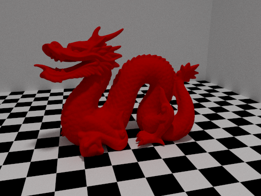
Scene 1: Stanford Dragon: 871K triangles, in axis-aligned orientation

Scene 2: Robot: 1.6M triangles, at 45-degree rotation to axis-alignment

Scene 3: XYZ Dragon: 7.2M triangles, axis-aligned orientation

Because of the fact I’m using a two-level hierarchy of acceleration structures, in order to test Scene 2 fairly with regards to the axis alignment rotation, I’ve re-baked out the mesh in world-space with a 45-degree rotation around the Y (up) axis, so that its triangles are rotated within object-space as well.

KDTree leaf node threshold size is always 6, and for min/max binning approximation, when the number of objects left to be split is less than 8192, I switch over to the normal “Greedy” implementation - otherwise, I’ve found that min/max binning does a pretty poor job of splitting at that level. Published papers on the min/max binning algorithm for KDTrees seem to show similar issues.

In terms of recording the specific times, this is being done within the code using gettimeofday() to record the respective start/end times, calculating the difference and convert it to double precision, giving a number in seconds. That number is rounded to 5 decimal places.

For all test configurations, I’ve run six independent tests in a clean state, and the results shown here are the mean average of those results, again rounded to 5 decimal places. For the last two tests of Scene 3, there were differences in time for some of the tests outside the margin of error, so I ran a few more tests for those. The tests were all run on the same computer (Dual Xeon, Sandy Bridge micro-arch), running Linux 3.5 kernel, and all test executables were built with GCC 4.7.1 with the same options. I also tried to ensure that the CPU core temperatures were below 60 degC before running each test.

Test Results / Analysis

Scene 1

With min/max binning approximation, build times are relatively fast (a fair amount of the time is taken up by the “Greedy” partitioning which takes over after 8192 triangles), and surprisingly, while checking all three axes instead of just the single largest extent axis takes longer, it doesn’t take three times as long, which is what I would have expected. I guess some of the time would be due to memory allocation, which when checking all three axes is only done once.

On the rendering side, the fact that all axes were checked while building seems to have very little effect in this case, indicating that the extra time penalty for building might not always be worth the effort. Enabling Inverse Hashed Mailboxing has a huge effect on render times, effectively reducing the render times to ~73% of their previous times.

With the “Greedy” n log n partitioning method, build times are more expensive, and the “Empty bonus” value, used when building to maximise - or cut away - empty space has a very big effect on both the build time and the render time. Based on the memory allocation numbers I noted, and thus the number of nodes in each KDTree, I can see that having a bigger empty bonus leads to deeper (and therefore bigger) trees, as expected, but also better rendering times. Checking all three axes gives slightly better render times with an Empty Bonus of 0.9, but worse render times with one of 0.5. Triangle clipping is very expensive at build-time in this test, and only provides slight speed improvements at render time.

Although faster to build, the min/max binning approximation cannot generate trees as well as the “Greedy” one, so render times are significantly faster with trees built with the “Greedy” method. Once again, Enabling Inverse Hashed Mailboxing significantly reduces render times across the board.

Scene 2

Min/max binning really struggled with this mesh, not really partitioning the triangles very well, and leading to very large leaf nodes (over 400 triangles in some cases) once the depth limit (35) had been hit. Checking all three axes gave barely detectable improvements at render time.

Again, Enabling Inverse Hashed Mailboxing has the same effect as seen previously.

Once again, with the “Greedy” partitioning method, build times are more expensive, but with this mesh, a more aggressive Empty Bonus value produced deeper trees with no benefit - I think this is down to the fact that the mesh has been rotated at 45 degrees to the axis alignment, leading to non-tight AABBs. This is backed up by the fact that the tests with “Clipping” enabled (which spatially clips triangles to test split criteria as well as clipping a node’s BB to its parent node’s, thus removing overlap) not only build faster despite doing more work, but have significantly reduced render times. Checking all three axes in the final test with clipping enabled is much more expensive at build time over testing a single axis, but gives a reasonable render time improvement.

Once again, Enabling Inverse Hashed Mailboxing significantly reduces render times across the board.

Scene 3

In this test with min/max binning, checking all three axes has a fairly moderate penalty at build time over checking only one axis and provides a very slight render time improvement. Enabling Inverse Hashed Mailboxing provides a significant render time improvement once again.

The “Greedy” partitioning method takes a significant amount of time to build with this mesh, sometimes taking longer to build than it does to render (although building is single threaded as I’ve disabled multi-threaded building). Except for a strange result with the test with Empty Bonus of 0.5 and checking all axis, which for some reason produced huge trees (based on the number of nodes allocated) but still with large leaf nodes, leading to slow performance, the same general picture appears, although this time the “Empty Bonus” variable has much less of an effect, as does the clipping and checking all axes. This is probably because with this mesh it is axis-aligned in general, and the triangles are extremely small. Based on the build-time penalty for clipping and checking all axes, the pay-off for build-time vs render time in this test doesn’t seem as worth it.

Inverse Hashed Mailboxing once again brings down the render times in all cases.

Conclusion

KDTree building is very expensive, especially with “Greedy” n log n building, but in all cases this generates faster trees for rendering than min/max binning approximation does. The “Empty Bonus” variable seems to have variable results, with more aggressive values giving deeper trees but faster render times for some meshes, but producing worse trees in other cases. With “Perfect Split” clipping enabled, build time is even more expensive, but with meshes that don’t have tight AABBs, seems to be well worth the extra work. Checking all axes doesn’t really seem to provide that much benefit, but with min/max binning, it’s possible to parallelise checking all three axes at once with SSE intrinsics, so the cost/benefit payoff is possibly there, although that’s not possible for KDTree building with the “Greedy” method or when spatially clipping triangles, so standard scalar code needs to be used, increasing the work that needs to be done.

Using Inverse Hashed Mailboxing provides no build-time penalty and significantly reduces render time in all situations.

Future investigation: Given how much better the results of KDTree building are with “Greedy” building, I’d be interested in what benefit using min/max binning over standard binning has with BVH acceleration structures, and whether the huge potential penalty for doing “Greedy” building with BVHs would provide any render time benefits.

C++ Virtual Function Overhead

I have recently been trying to change Imagine’s Acceleration Structure infrastructure to be more dynamic, allowing different objects and geometry instances to have different acceleration structures either automatically based on heuristics, or based on user-specification within the interface.

Imagine’s acceleration structures have for the past two years been implemented with the Curiously Recurring Template design pattern, which allows virtual function-like ability to some extent while enabling the compiler to inline the functions. I chose this way of doing things as I had assumed that Virtual Functions would have some overhead, despite previously doing some experimentation with Virtual Functions and surprisingly finding they don’t seem to have any overhead compared to fully-inline-able functions.

The “Curiously Recurring Template” pattern doesn’t easily allow a templated base class (for Triangles, Shapes or Objects in Imagine’s case) to be specified as a pointer and then the actual implementation to be instantiated as a derived templated acceleration structure, which is what I needed for this dynamic flexibility.

So I decided to do some more benchmarks to investigate any overhead again.

First of all, I tried a synthetic benchmark of just a simple for loop of 1,073,741,824 iterations, calling getHitObject() on the acceleration structure pointer. For the “Curiously Recurring Template” implementation, the pointer type was of KDTreeVolume<T>, the actual derived class and the object allocated for that pointer was of the same type. In the Virtual Function implementation, the pointer type was to AccelerationStructure<T>, the base class and the actual object allocated for the pointer was KDTree<T>, a duplicate of the KDTreeVolume<T> class but which used standard C++ virtual inheritance from the abstract AccelerationStructure<T> base class. The code was run in a single thread.

Eight pairs of runs were done, alternating each implementation, and I tried to make sure the CPU core temperatures were under 55 degC before starting each test to ensure that there was no disadvantage to be had by a core not being able to Turbo Boost overclock.

Other than the first two results for the “Curiously Recurring Template” implementation, the Virtual Function method seems very slightly slower, but this difference is within the margin of error. This surprised me, but given the simple test case, it’s possible that the processor’s branch-predictor was negating the overhead of the v-table lookup, and thus might not be showing the difference.

So I decided to do some more realistic general purpose rendering benchmarks with the two different implementations, to see if any difference could be spotted there.

I created a scene with a fully-enclosed room, with 32 cubes inside and 2 area lights, and all surfaces fully diffuse. All geometry objects had less than or equal to 12 triangles, so the acceleration structures would be very shallow and thus any Virtual Function overhead would not be dwarfed by the work each function was doing on the acceleration structure.

The first test was at 1024x768, with 256 samples per pixel, and 10 ray bounces. With this test, the getHitObject() function would be called 2,013,265,920 times (for each camera ray and each diffuse bounce ray) and the doesOcclude() function would be called 4,026,531,840 times, once for each light (no light importance sampling was used) for each surface evaluation. All threads were being used for rendering.

The above results are in minutes, and show that the Virtual Function implementation was consistently slightly faster. I decided to do these tests again with double the number of samples per pixel (to double the above numbers), and again the results were pretty much the same:

I’m still surprised by this, but I’m putting it down to either compilers being a lot more clever than they used to, or the inlined “Curiously Recurring Template” implementation creating bloated instruction size. Or more likely, the fact that things like cache misses, load dependencies and branch miss-predictions within triangle and boundary box ray intersection code hide any overhead there may be.

Regardless, it appears that to all intents and purposes in my use-case, Virtual Function overhead is practically non-existent. I’m sure things would change with deeper inheritance hierarchies and multiple inheritance, but at least in my use-case it seems safe to move back to Virtual Functions. What’s more, Intel’s Embree high-performance ray tracing kernels use Virtual Functions, and they’re pretty-much state-of-the-art.

Accurate Ocean Waves

I’ve now implemented the ability to create geometry for accurate open ocean waves, based on Jerry Tessendorf’s “Simulating Ocean Water” paper.

This is orders of magnitude more realistic than the previous hack effort I did (see previous post), and accurately models wave and wind interaction for very accurate wave shapes, specifically the tapered crests of waves.

(Barely) Plausible Wave Displacement

I’m on holiday on the South coast this week, and after amazing weather, this morning it’s had the audacity to rain, so I thought I’d see how difficult it would be to make a fake-but-sometimes-plausible procedural texture for emulating waves on the sea via displacement.

Jerry Tenssendorf’s paper “Simulating Ocean Water” is essentially the way to do it accurately, using a discrete Fourier Transform, which allows very accurate modelling of wave peaks and troughs based on the wind interaction and gravity, and indeed other waves around them.

I only had a couple of hours I wanted to devote to it, and couldn’t get into that level of detail, so I tried to fake it by just using Simplex noise modulated by the sine of the texture coordinates.

Basically, at a very simple level (ignoring wind which is pretty important for accurate simulation), the peaks and troughs of waves on the sea closely resemble a trochoid, which can be emulated with the sin() function. I ended up modulating two different resolutions of these waves (major primary waves and smaller secondary waves) on top of each other along with noise, which at least for non-open-water waves (open water waves crests tend to have angled peaks when it’s windy and when the number of waves increases) with moderate wind, gives reasonable results. It’s certainly better than just random noise. But it’s very rigid and consistent even with the noise modulation, so for large areas it basically looks like a tiled texture.

At some point, I’d like to investigate implementing Jerry Tenssendorf’s paper to do it accurately.

Oren Nayar BRDF

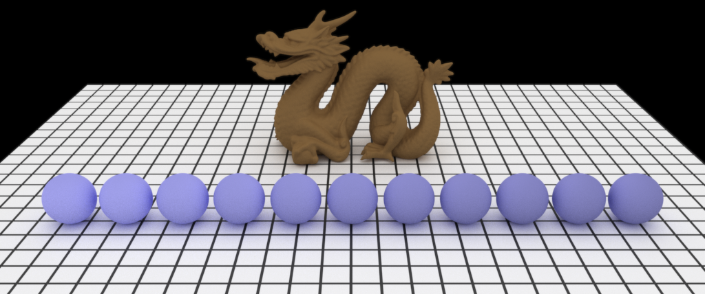
I’ve had this code kicking around for ages, but it never worked correctly, due to a bracket in the wrong place! Finally got it working, so Imagine can do realistic diffuse rough surfaces like clay.

The image below shows spheres with incremental roughness values, and a terracotta dragon.

Animations

I’ve been messing around with simple animations rendered out of Imagine recently, and I’ve put some of them up on Vimeo:

Robot Instances:
Full Video

Depth Of Field:
Full Video

Displacement

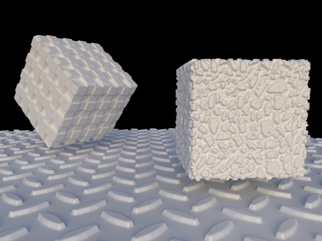
I’ve now added initial support for displacement of geometry after subdivision using displacement maps. It’s far from perfect yet - it’s quite slow when subdividing to the number of levels required for decent results (the two cubes above are 6.2m faces, subdivided 10 times), and the Half-Edge data structures I’m using for subdivision use a fair amount of memory, and there’s a very slight amount of faceting that doesn’t look normal.

The first two issues (speed and memory consumption) I can probably fix quite easily by making my Half Edge data structures more compact and efficient - currently, each Half Edge Vertex, Half Edge Edge and Half Edge Face store pointers to each other which while easy, consumes more memory than required. Converting them to using offset indexes (like my KDTree does) should bring memory usage down by half (instead of storing an 8-byte pointer, it’s possible to store a 4-byte uint_32 for an offset into a table).

It’s also not on-the-fly micro-polygon displacement - that’s more difficult (and slower while rending), can only be done on triangles (loop SubD is the normal variant) but uses much less memory and allows easy adaptive stopping criteria by checking each edge length in camera-space to see whether it’s smaller than a pixel yet.

There’s also vector displacement (displacement in three dimensions, as opposed to simply along the vertex’s normal), which should be pretty trivial to implement.

Subdivision

Imagine has had support for Catmull-Clark subdivision of quads within its interface for a while now, but the previous implementation had several limitations: it was slow and memory-inefficient (it just brute-forced the subdivision from the original faces), it didn’t support open shapes with holes and it didn’t keep UVs.

I’ve now re-written this to use a half-edge mesh structure, which makes it faster (less duplicate work is done), it supports boundary edges (holes in geometry), supports triangles and it subdivides UV positions (linearly at preset). I’ve also added support for linear subdivision with no smoothing.

Once I sort out the Geometry Instance infrastructure for each object in order to allow Geometry Modifiers at render time, it should be fairly simple to add Displacement support.

Wireframe Shader

Discussion at work led to talking about implementing a wireframe shader in Nuke, so I decided to see how difficult it would be in Imagine. As long as the mesh consists of polygons of a single type - i.e. triangles or quads: not difficult at all it turns out.

For triangles, it’s easy enough to emulate a wireframe surface by simply working out how close a hit position on a triangle is to an edge by transforming the triangle’s points into world space and then using the standard point-to-line method of a perpendicular vector to each edge. This gives you the distance in world space of the hit position to each edge, and based on which distance is the closest, you can then apply a step function to the colour of the surface, based on the distance and a line thickness amount.

For quads, I first tried using the same algorithm as for triangles, but ignoring the edge of the triangle that was shared within the quad. This worked to some degree, but each quad had two opposing wedges in the corners where the point-to-line formula meant that parts of some edges weren’t shaded correctly.

So instead, I decided to use the Barycentric coordinates of the hit position within the triangle. This allowed me to correctly isolate all four edges of the quad based on a fixed threshold, but I then had to work out the line width and keep it uniform to the length of any edges. In the end I multiplied the Barycentric coordinates of both the the hit position and the inverse hit position (for the opposing edge of the quad) by the length of each of the non-shared edges of the triangle, giving a distance. The smallest of these distances I then used to step the colour, as I did for triangles. While this might not be perfectly accurate and work in all situations, it seems to work very well in practice and also allowed me to (almost) match the line thickness to the triangle method. It also looks very nice:

There’s a very slight (~1%) overhead in shading, as triangles have to be fetched and transformed to world space, but both of the renderings above at full HD finished in under six minutes with 676 samples per pixel.

When I sort out the texturing infrastructure to make it more flexible, it should be very easy to apply this texture as an alpha texture for a fully-3-dimensional mesh that is able to be seen through and cast shadows.