I’ve spent a fair amount of time over the last three months following through the second part of Robert Nystrom’s fantastic Crafting Interpreters free online book, consisting of a complete step-by-step guide to how to “craft” a complete and fully-functional interpreter language virtual machine.
I made an attempt to start two years ago on the tree-walk version, but didn’t have the motivation at the time to complete it (I think the fact I knew the bytecode VM version would be better and more useful/interesting subconsciously made me not bother as much given the bytecode VM version’s chapters were still being written), but I realised just before Christmas that the book had been complete for a few months now, so made a bit of an effort to find time to complete it by writing my version based off the book, as I had a use-case for scripting language embedding in some of my apps that I thought having my own language/VM for could be quite useful/interesting.
I’ve enjoyed the process of following along, learning and writing my own version immensely, and I now have a version - called “Mint” - which is heavily based off the book, but with some subtle language syntax changes and written in C++ instead of C (not sure yet whether that was the best idea in the end, although I hope having a namespace might be useful for embedding in other codebases), and has several additional features over the stock book version of ‘Lox’, for example:
Built-in dictionary/map variable type support for key/value lookups and storage
Support for compound assignment operators (+=, *=, etc)
Array/list slicing / assignment support
break and continue loop-control syntax support
Support for multi-line comments (C/C++-style) and both “#” and “//” single-line comments
Ternary ? operator syntax support.
Example code listings, demonstrating fizzbuzz:
// fizzbuzz

for (var i = 1; i <= 100; i += 1)
{
	if (i % 15 == 0)
		print "fizzbuzz";
	else if (i % 3 == 0)
		print "fizz";
	else if (i % 5 == 0)
		print "buzz";
	else
		print i;
}
Calculating the approximate value of PI:
# calculate PI with the Leibniz algorithm...

def calculatePI(iterations)
{
	var x = 1.0;
	var pi = 1.0;

	for (var i = 2; i < iterations + 2; i += 1)
	{
		x *= -1.0;
		pi += x / (2.0 * i - 1.0);
	}

	pi *= 4.0;
	return pi;
}

var piVal = calculatePI(40000000);
print "PI: " + toStr(piVal);
producing:
PI: 3.14159266192262
and a fully-functional Mint Class, which can convert Roman numeral strings to numbers and vice versa, downloadable here
I’m going to continue developing it in the background, in order to attempt to integrate it into several of my applications, and also try and optimise its performance a bit and see how it compares to other interpreter languages.
A year ago I started writing a new basic app (Sniffle) to find log files based off directory/filepath patterns, allowing for recursive directory pattern wildcard matching, and then performing file content operations on the found files, mainly involving grepping/counting items, with an emphasis on finding files on NFS networks. Existing applications like grep, ack and ag (amongst others) do provide existing functionality for some of the use cases, but their defaults are generally wrong for my use-cases (i.e. I want symlinks to always be followed, and to do recursive searching by default), and some of the methods they use to be fast are not always directly compatible (at least efficiently) with NFS networks (i.e. mmap-ing files for better content searching performance).
The number of logs I’d want to search through was often in the tens of thousands, and some of the logs are (unfortunately, and often needlessly) very verbose and can be > 5 MB in some cases. Using a log database or some other similar infrastructure would generally be the more principled way of solving this issue at scale, but I’m generally the only person who occasionally needs to perform these searches, so getting dedicated infrastructure (i.e. a database) for this use-case from IT was very unlikely, essentially meaning I ended up writing my own solution at home in my own time for use at work.
I’ve had working support for finding files, grepping through those files, counting string matches in files and finding multiple cascading strings (optionally in particular orders - i.e. if the first one isn’t found, there’s no point looking for any of the others) for a while now, as well as the ability to filter the list of found files to grep/process first by modified date (e.g. log files last modified within the past 5 days) or file size threshold, but a new use-case came up at work recently where I wanted to look for time period gaps in the log timestamps, indicating that the process writing the logs (a renderer) either hadn’t been doing anything for a while, or had taken longer than expected to do some task.
Checking the time delta between timestamps on consecutive lines in a file is pretty trivial to implement at a conceptual level, however doing so in a way which is performant is a bit more work: naively using strptime() to parse the time has a significant and noticeable overhead, due to internal use of mktime() which is very expensive, and even using sscanf() to pull out the constituent parts and rebuild them, or using a series of atoi() calls - while noticeably faster than strptime() - can be improved upon if you’re just extracting digit components in known positions (although supporting multiple date-formats complicates this slightly).
Given a fixed and valid timestamp string with consistent width zero-padding - which I could validate and guarantee in my use-case - I ended up settling on subtracting each string character value per timestamp unit digit by the char value '0', to give the 0-based 0-9 integer value, and then multiplying it by its digit position in the component number and adding these values together grouped by component number, effectively extracting and accumulating final values very quickly.
It’s somewhat hacky and verbose, but demonstrably faster than the more normal approaches mentioned above, which for my purposes made it a worthwhile optimisation.
As an example, given a std::string currentString; representing a non-empty log line which is guaranteed to have at least the minimum number of string characters for an ISO 8601 date/time stamp, and size_t timestampStart representing the character position offset within the string where the timestamp starts (in order to support varying formatting around the timestamp), with the start of a log line looking something like this:
[2019-03-22 09:42:13] Did something useful
then code to parse the year from the string looks like this:
and handling the time components is done similarly with appropriate position indices.
Using these component integer values to represent a full time value is now context-dependent on what’s trying to be achieved: if you just wanted to sort the timestamps, you could just accumulate the numbers, multiplying each component by a component-respective multiplier to build the number of seconds, i.e.:
In other words, using a constant of 31 for the number of days in all months: because we’d only care about relative positions based on numbers for sorting, and not absolute deltas, it wouldn’t be necessary to use the correct number of days in the month.
However, for the use-case of working out time durations between each log timestamp, absolute delta values are required, and this does involve knowing the number of days within each month - so that you accurately know the difference between 23:55 on the last day of a month is 10 minutes before 00:05 on the first day of the month, which makes things a bit more complicated. I ended up using two pre-calculated static const arrays of the months,
one for non-leap year years, the other for leap year years, i.e.:
// pre-calculated totals for numbers of days from start of year for each month
static const unsigned int kCumulativeDaysInYearForMonth[12] =			{ 0, 31, 59, 90, 120, 151, 181, 212, 243, 273, 304, 334 };
static const unsigned int kCumulativeDaysInYearForMonthLeapYear[12] =	{ 0, 31, 60, 91, 121, 152, 182, 213, 244, 274, 305, 335 };
and then working out whether the year was a leap year by cheating a bit and only checking the first timestamp on the first line of the logfile to see if it was a leap year, and then caching that in a variable for the rest of the log processing:
which then meant not needing to do any branching for any of the remainder log line timestamps to work this out, and being able to build up the number of seconds
a timestamp represented with:
which then works to provide exact absolute counts of the number of seconds the timestamp represents for nearly all situations, except for two:
The first line of the log file having a timestamp almost two months before the end of February, e.g. December 30th, and some following log line timestamps in the same log file then progressing on to the end of February, potentially meaning there was a discrepancy between the code thinking the year was a leap year or not
Daylight Savings Time changes
Both of these situations in the end I decided to ignore: the first one because it was a total non-issue for my use-case, as if the length of the log files timestamps stretched to almost two months, straddling a new year and then on to the end of February, there would be much bigger issues to worry about: almost all log files should have had a duration of under 48 hours, and anything over two weeks long would be a pathological situation.
For the Daylight Savings Time change, while it was a definite potential issue that could happen - either adding an extra hour or removing it from the time value in the hour after the change - which could then have tripped or not tripped the time delta threshold logic incorrectly, I was happy to let that problem slide: dealing with DST changes in computer systems is almost always problematic in my experience (especially if using local timestamps like here), and while it was technically solvable if you know the dates it changes (per geographic location: different countries change at differing times during the year, and the Earth hemisphere matters as well for direction), I just didn’t feel it was worth it for the potential of some false positives/negatives happening within two to three hours per year.
Over the past year I’ve been working on (and to a much greater extent optimising) an image texture cache system for Imagine.
Imagine has had some form of reading planar (entire) images since very early on, but other than a slightly hacky integration of OpenImageIO (but that did work efficiently) into Imagine just to test things, it hasn’t had proper integrated support for reading (and more importantly paging) partial images lazily on-demand. This ability is essential for a production level renderer in VFX, as the size and number of image textures used in VFX for rendering is pretty extreme.
I could have just integrated OpenImageIO properly into Imagine, but there were a few reasons I didn’t want to do this: First and foremost, I wanted to write my own and experiment with different ways of handling concurrency, scalability as well as eviction. Second, I already had my own file readers / writers and didn’t like some of OIIO’s dependencies. Further reasons were that OIIO comes with a fair bit of baggage which at least in my use-case for texture reading, I didn’t care that much about: in particular rather bloated data structures in some cases (partly due to Field3D support requiring matrices). It also had some limitations: didn’t support constant tiles, although in fairness there aren’t any open file formats that support this, although I’d like to investigate creating a file format at some point - which can make a huge difference in terms of File I/O bandwidth (which is a very important bottleneck for high-end VFX rendering), it doesn’t natively support texture atlassing (e.g. UDIMs) and I was also not completely convinced by its efficiency or scalability, although it definitely is a capable and production-proven library. I also wanted to experiment with adding new features like on-the-fly compression of tile data, and doing this in a clean and minimal code-base would be much easier.
Imagine already had file readers, but they only supported reading planar images into image buffer classes, so the first step was to provide the ability for a file reader to describe the metadata of an image file, and fill in the details, including resolution, number of channels, data type and mipmap levels.
In terms of general storage of image textures, I created something that’s essentially similar to OpenImageIO’s overall design, whereby there are two main items stored in the cache: image items, which represent the actual image file metadata, and image tiles, which represent the pixel data of the images themselves, broken into small tiles. However I wanted to try slightly different algorithms to what OpenImageIO uses for tile eviction, as I had the suspicion the method it uses (mark and sweep iterator over entire tile cache) wasn’t the best approach from a speed and scalability perspective. One of the ideas I had in mind was not actually removing any tile items at all at eviction time, but only freeing the pixel data itself. This would use more overall infrastructure memory (excluding pixel data), but it should reduce the need to lock the entire tile cache very slightly, which hopefully would help scalability and performance. Given that classes and structs representing texture items and texture tiles would never be freed at tile eviction for paging, it was therefore extremely important that they be as memory efficient as possible.
I made a conscious decision to not separate different channel images based on tiles requested based on the channels requested - that is, if an RGBA image was loaded, but only the A channel was requested, I’d still load all four channels into memory instead of partitioning each tile and having an extra dimension to have to cope with for the tile hashes. This was partly to keep things simpler, but also to constrain the number of tiles given I wanted to not have to free the tile items at all when paging, only freeing the pixel data. It would mean however, that in certain situations like the example given above, memory usage would be higher than needed. However, as is generally done in high-end VFX, the solution here is to make sure each texture image just contains one set of channels, so the above example would have two textures, one for the RGB channels and a separate one for the A channel.
I also made a decision to not use lazy texture loading for HDRI environment maps, but to keep those separate, partly because you’re effectively point-sampling them anyway (definitely at construction time to build the CDFs), but also to keep texture requests down for this type of illumination.
I also wanted to be able to categorise images based on purpose, both for allowing different caching / eviction strategies for different types and to allow different types of filtering to be done on them: there are some situations like for alpha/presence maps and layering mask/mix maps that it’s generally better to err on the side of less filtering, even at the expense of possible aliasing.
To begin with I started with just the bare basics as I wanted to investigate and experiment with different ways of doing things to see the effects they would have. As a starting point I initially just had a single mutex around each map collection, so that I could see what the extreme worst-case scenario was.
Imagine was using ray differentials to calculate texture filter regions and thus the mipmap levels to pull in of the textures, and doing trilinear filtering to combine mipmap levels.
Tests even with just a single plane polygon in the scene with one texture were as expected pretty abysmal, with CPU utilisation on a 16 core / 2 socket system hovering around 300% (instead of the ideal of 1600%).
I implemented per-thread microcaches that stored LRU arrays of pairs of both the texture items and their hashes and tile items and their hashes, which was used to lookup textures before going to the main cache and in this contrived scenario, other than for the first few buckets where all threads were initially opening file and reading images, CPU utilisation went up to the expected 1600%, fully utilising the available cores.
Testing with other simple objects added to the scene with the same texture (so that there were now indirect rays being fired in an incoherent fashion) could scale to a degree if I increased the microcache sizes, but this wasn’t going to be a good approach, as the single mutexes around the individual map containers were clearly the bottleneck.
So I needed to come up with a solution which would scale well with many threads. In the end I settled on writing my own map container wrapper similar to Java’s ConcurrentHashMap (which is also similar to what OIIO uses, and how Linux’s hashed spinlocks work), which splits the map into different “bins” (although I called my version “shards” which is more in mapping to the database partitioning technique). Each “shard” contains its own isolated map and mutex, and the shard to use for lookup and inserting values is chosen by using the modulus of the hash value for the key, based on the number of shards. It’s then possible to lock just this shard and lookup within its individual map to find / set the value as required, while other concurrent requests from other threads will have no contention, so long as they map to different shards. If they do map to the same shard, then there will be a certain amount of contention. So it’s extremely important to have a very good hash function which distributes well over the domain space. In my case, after an awful lot of trial and error and playing around with the avalanche effect of hashes for tiles, I came up with hashes which seem to work quite well: I used Austin Appleby’s MurmurHash3 for hashing the filename, generating a 32-bit integer, which allows lookups of the texture item itself.
For tile items, I ended up using a 64-bit integer of the 32-bit texture item hash shifted 32-bits to the left, being added to by the mipmap level shifted 24-bits to the left, then the tileY coordinate shifted 14-bits to the left with the final tileX coordinate unshifted.
Another very important factor which was important is mixing the hash used to lookup the shard so that it doesn’t have the same correlation within the shard’s hash map, which can severely affect the efficiency and load factor of hash maps within each shard.
With this implementation, scaleability was perfect on 16 threads with these simple scenes, so I then attempted to stress-test it with more complex test scenes and finally as close to a production level scene as I could fabricate texture-wise.
I tested initial scalability of the locking by using “virtual” image texture readers which just generated texture colours procedurally (tiled based) so as not to be limited by disk speed or OS-level disk caching.
Tests with the extreme worse case scenario (just a single mutex around the containers - and using the less-than-ideal std::map<> to begin with for lookup structures) were understandably atrociously bad, although interestingly scaling on Linux was much better than on OS X, probably due to Linux’s Futexes.
Scalability with sharded maps was much better on OS X, and noticeably better on Linux, scaling close to linearly with 32 shards for both maps. Changing the underlying map type to std::unordered_map (hashmap) reduced lookup time by around 25%, which was not as much as I had hoped. I experimented with setting the initial bucket count and max load factor for the maps and this reduced lookup time by around 10% again, and at this point I was slightly worried that my hashes weren’t as well distributed as I thought - so I thought this would be a good time to both check the distribution of the hashmaps and see if the strategy of not deleting items from the maps gave any benefit. Without controlling the load factor and initial bucket count, once paging started happening, not deleting items seemed to give a slight speedup - possibly due to the fact tombstones didn’t need to be used to mark items as deleted. However when optimising the initial load factor and bucket count, the difference was negligible - probably due to hashes mapping very nicely to open buckets with very few collisions happening. However the ability to not delete tile items did mean that in the texture stats I was able to very accurately track unique texture data read during paging, which is quite useful, and I kept this as an option.
I experimented at this point with increasing the microcache sizes a bit (to 16 entries per thread for both), and for simple scenes with less than 60 textures this made a noticeable difference (especially with paging enabled, as it meant if an item was in a microcache it was recently used so it shouldn’t be evicted), but once each ray hit was evaluating more than 10 textures for layered materials, these microcaches became barely useful due to almost random thrashing between vertices per path. I have some ideas for trying to use more tree-like data structures for them in order to take advantage of ray-tree coherence, but the best approach here would just be full-on deferred ray batching / sorting, so I’m not convinced it’s going to be worth it.
At this point without having to page textures to fit in a particular memory limit, my texture cache was faster than OpenImageIO for pretty much identical numbers of texture evaluations, but with aggressive paging turned on OpenImageIO was noticeably faster. Looking at the stats between the two, it was obvious that my naive eviction method was causing an awful lot of duplicate reads (still using virtual file readers, so no disk access was taking place, only memory allocations and procedural textures). I decided to just copy OpenImageIO’s clever method of marking a tile as recently used with an atomic variable, allowing a very cheap compare-and-swap to be done, allowing skipping recently-used tiles very accurately and efficiently, although with a slightly less cumbersome mark-and-sweep process. This change made a huge amount of difference, with my texture cache now being ~5-10% faster than OpenImageIO. I also experimented with over-evicting based on a ratio to prevent continual locking: if a request for a new image needed 2KB of data, I’d actually free more than that, so as to do more work within the one lock event meaning it would be more likely the next request for a new texture would not need to lock as well to evict - this made a noticeable improvement (after experimentation I settled on doubling the target eviction size).
I then decided to move to proper tiled based image textures, testing both TIFF (briefly) and OpenEXR. I noticed immediately with OpenEXR that using the worker thread calling OpenEXR to read images (i.e. with the threadpool size set to 0) had severe contention issues, caused by redundant locking in IlmBase’s ThreadPool class. Larry Gritz had also spotted this issue previously and had a fix for it on GitHub which allowed EXR reading with worker threads to scale a lot better. Along the way of testing with bigger and bigger scenes I had to fix several issues with ray differentials not propagating correctly causing incorrect point-sampling of the lowest level mipmaps, which obviously slows things down to a halt. In the end for some edge cases I had to build in texture filtering based on approximate ray-width as a backup for when ray differentials failed (due to incorrect/inconsistent UVs or missing UVs on meshes).
I then decided to scale things up to an extreme test to stress test the cache: I tested with a large cornell-box style scene containing four production-scale hero objects - many different components with different materials, all with UDIMed textures with varying numbers of layers (one to three, controlled with mask textures controlling mixes), with diffuse, specular colour, specular roughness, clearcoat reflection and bump textures being utilised for most (but not all) materials. The floor and the walls of the Cornell box also had diffuse textures of 10x10 tiles of UDIMs (so each plane other than the ceiling consisted of 100 texture files).
The total number of image texture files was 898, and I made use of OpenEXR format tiled mipmaps of 16-bit half format at 8K, the tile size being 32x32. Total size on disk for all textures was over 320 GB.
I tested with path length set to 6, so there would be a large amount of incoherent texture accesses.
Testing this scene showed it worked very well, and was consistently slightly faster than OIIO - this is probably partly due to less locking that I do in general, but probably also because my texture cache has full integrated support for UDIMs, so can batch up requests to adjacent tiles on UDIM borders and when filtering to reduce locking even more.
I experimented with adding support for compressing pixel tile data in memory using LZ4 - the idea being that for constant tiles (which no open standard tiled file format supports at present, so there’s no way to detect them up front) it might be a way to detect these on-the-fly with a tiny bit of overhead. Testing with simple textures worked well, and if the compression ratio was excellent it was obvious it was a constant tile, and I could mark it as such and not bother evicting it, which brought a slight speed-up. If the compression ratio was just good, there was some constant data in the tile, and it meant I could fit more in memory without going back to disk when paging. However, with real-world textures painted in Mari it didn’t work as well, as outside the UV’d area Mari tends to distort texture detail instead of leaving it black, so there’s still texture detail there taking up space. One situation where compressing did still provide benefits with real-world textures was with layer masks texture maps used for mixing / isolation, which are generally less detailed anyway - it was possible to often detect constant tiles and even if there weren’t entire constant tiles still compress image data usefully within tiles.
So I now have a very fast, efficient and scalable image texture cache - I still think there could be better texture formats than OpenEXR which unfortunately has become the standard for textures at VFX level but is seemingly somewhat abandoned: OpenEXR’s threading is really bad, and the use of threadpools doesn’t really make sense for reading multiple random tiles per random mipmap level in parallel in a path tracer - it’s possible with coherent access using threadpools is still a win for rendering (it definitely does make sense to use threadpools to speed up reading a single large entire image for use in image viewers and compositors, and for writing images), but I think it makes sense that a file format for rendering be completely stateless, with metadata decoded once, and then any number of threads be able to read/uncompress at will without dependencies / state controls - obviously depending on how the image is compressed there may be problems here, but a balance needs to be found. In addition OpenEXR doesn’t support 8-bit or 16-bit integer formats which can be very efficient for certain types of data (masks / isolation maps), neither does it support constant tiles or instanced tiles. So I’m tempted to try creating a texture format just for rendering, optimised for extremely fast random access.
I ended up spending a fair amount of time on the Katana integration in the end, at least in terms of pulling in geometry attributes and static transforms and exposing materials, so that I could pull production scene geometry into Imagine and see how well it coped against the latest versions of PRMan and Arnold. Initially, before I started work on memory efficiency back in June, it was embarrassingly bad, with Imagine using around 9-11 times as much memory, and Imagine only being able to fit around 52 million unique triangles in 24 GB of RAM. In this original state, Imagine was using gathered vertex attributes, so there was a lot of duplication of data.
The first thing I did was to add the ability to use indexed vertex attributes, and this way the source attributes (points, normals, UVs, etc) could be shared among any triangle / vertex in the mesh, with “just” indices being used to index into them. I put “just” in quotes, because vertex indices can also require a lot of memory, especially if the indices for each attribute are different (i.e. points, normals and UVs all have different indices per vertex).
This change reduced memory usage by around 3 times, but it was still not great. I added logic to detect if certain attributes used the same indices (i.e. normals and UVs), and this allowed me to re-use/share indices for multiple attributes if the indices allowed that. The next thing I experimented with was de-duplication of vertex attributes. In a normal closed mesh consisting of quads, the majority of points, normals and UVs are shared by multiple faces, and annoyingly, DCC tools like Maya don’t seem to put much effort into de-duplicating these attributes (other than points) on export (possibly due to the fact that some renderers like PRMan don’t support specifying indexed attributes explicitly at ingestion stage), so UVs and smooth normals values are generally specified up to 2/3 times. Doing this de-duplication (of normals and UVs) added to the startup/build time cost (as well as the peak memory usage), but did reduce overall memory usage quite significantly - sometimes by as much as 40%. However, it came at an additional cost, in that the indices for each vertex attribute would now be totally different and couldn’t be shared, so while the memory usage for the raw vertex attributes themselves was now less, a bigger percentage of the memory usage was now being used by the indices themselves.
Changing the infrastructure to allow indices to be specified as uchar (1 byte), ushort (2 bytes) or uint (4 bytes) depending on the number of attributes of a particular type there were as well as allowing sharing of indices brought more flexibility and efficiency for smaller meshes (but at the unfortunate cost of some rather nasty template type logic in the code), however memory usage was still around 3.5-4.5x more than Arnold and PRMan for the same geometry, and peak memory usage was even higher during build time for de-duplicating normals and UVs.
I had been using 48-byte triangles (on top of the vertex data), based on the fast Shevtsov, Soupikov, Kapustin intersection algorithm which caches several things like base points, edge lengths and overall normal for each triangle, without having to do a lookup into the mesh vertex attributes themselves to do the intersection test - however this was using far too much memory (especially for deformation motion blur), so I added the ability to use several different possible triangle types dynamically per-mesh at build time, with the minimal Moeller-Trumbore algorithm being a new type which only needed 2-4 bytes (depending on number of indices items) of additional storage per triangle for the index into the indices for the triangle (I eventually got this down to 0 bytes extra by passing this index through from the acceleration structure).
This left Imagine using around 1.8-2.5x more memory than the latest versions of the other renderers, which while a significant improvement compared to the starting point, still left room for more. Due to the fact that there seemed to be a balance of memory used for raw geometry attributes vs the memory used for the indices into the attributes, with de-duplicating the attributes requiring a fair bit more memory for the indices themselves, the memory for both needed to be reduced at the same time.
I first investigated bit-packing the indices, but while doing this is fairly trivial when pre-computing / processing them up front (using delta encoding or high-watermark encoding), when completely random access is needed this becomes a lot more difficult. I experimented with hiword/loword encoding of delta differences between the indices for progressive triangles, and storing the indices for two triangles in one set of indices, but due to the variable nature of indices between adjacent values, it was difficult to provide random access without using some sort of keyframe-style encoding which got rather complicated. I realised that when vertex attributes like normals and UVs are fully specified - i.e. duplicates are given for each face, assuming that the attributes are listed in the order the polygon vertices are specified (in other words they aren’t indexed), then it’s possible to only store the base index for that triangle - the other two indices will either be the next sequential numbers (for triangles and the first triangle of a quad), or sequential after a gap of two shifted from the base vertex, with the final vertex being the base one for the second triangle of quads. I stole a bit from the item index to store the triangle type, and this allowed these indices to be worked out by only storing one value for all three indices for a particular vertex attribute. A further optimisation was realising that in certain cases (the mesh consisting fully of triangles or quads, or mostly quads with a very limited number of triangles) you don’t even need to store this base index fully - you can store the offset value after dividing the triangle index by a constant (which needs to be worked out before hand based on the type of mesh), meaning an 8-bit signed char integer can in certain (limited, but fairly common in general use) cases be used to store indices into the millions due to the indices of a polygon being consecutive due to the fact that shared attributes between faces weren’t being de-duplicated, so this base index is explicitly calculable on-the-fly.
These optimisations brought down indices memory usage significantly in the majority of situations, with no noticeable runtime penalty, but they relied on the fact that vertex attributes weren’t being de-duplicated.
So I then turned to trying to quantise non-point vertex attributes (point attributes need to be stored at full float precision due to FP precision requirements for the vast majority of general rendering situations, at least at VFX scale). It turns out there’s been a lot of research in this area, especially for normals, but a lot of it has been done with game engines / real time in mind. I first tried a naive compact representation of normals using spherical coordinates stored at half precision - using a total of 4 bytes instead of 12 bytes. While this brought down memory usage significantly, the accuracy was pretty bad and lossy, with axis-aligned directions not being fully reconstructable (for example 0.0,1.0,0.0 ends up being reconstructed as 0.000484,0.999999,0.000484) which is enough to cause shading issues.
Reading through the research on this subject (starting with Deering’s work in 1995 at Sun) did show that using full float (96 bits) representations was wasteful for normals: that’s accurate enough to shoot rays from the Moon to Mars with centimetre-accuracy on the surface of Mars (I’m assuming the relative positions of the planets makes a huge difference to this comparison!). In general (according to Meyer, Submuth, Subner, et el. in 2010), only 51 bits of floating point accuracy are required.
I tried a few non FP implementations of bit-packing at both 16-bit and 32-bit (because normals are unit length, you can just store two of the values and reconstruct the third): 16-bit is too lossy, but does allow storing axis-aligned directions losslessly, so might be useful for low LOD type situations where smooth normals were still required for some reason. 32-bit seems to work well, although you have to be careful about the distribution of the directions. It is obviously lossy, so comparing a normals AOV between full 96-bit precision and 32-bit packed does show differences, but in fairly comprehensive comparisons of beauty and other light AOV side-by-side renders, and worst-case test scenarios (extremely heavily subdivided sphere with heavy specular highlights, and the same sphere being perfectly reflective and reflecting a high-res checkerboard environment map light rendered at 4k square) and I’ve only spotted barely-perceptible minor differences in this latter test case. There’s a slight (just under 1%) overhead to rendering with 32-bit packed normals, due to three multiplications, one divide and a square-root being required to convert back to a full-precision normal. When using 16-bit packed normals an 8192 item LUT table can be used for the lookup, with no overhead at all. Using a LUT with 32-bit packed normals is unfeasible, as the LUT would need to contain 536M items, which is obviously ridiculous. For the moment I’m happy with this normal encoding, but there are more advanced and variable (in terms of size and precision) encoding methods with greater accuracy I could look into if I find accuracy isn’t good enough in the future. This change reduced normal memory storage down to a third.
Compressing UVs is more difficult, depending on what UV values you want to accept: using half format for each U,V value is acceptable in the range -2.0f - 2.0f, but outside of that, for any texture atlas usage, it’s too lossy, so for standard UDIM ranges (0.0f - 10.0f) just doesn’t work well with obvious stretching and differences, as the half precision just isn’t good enough at the bigger ranges.
In the end, I settled for a slightly hacky, but still generally very usable solution of compressing U,V values into 16 bits each - with a supported range of -10.0f - 10.0f - by just storing a scaled integer value of each value. I could double this accuracy by not allowing a full mirroring of the values below 0.0, but given as MPC’s v values are 1.0f - v, to render production assets I need this ability at least for the v value so I’d need to offset them, but that’s easy enough, and I so far have only noticed very minor artefacts from using this compression method when comparing against full-float UV representation with hero assets with high res (8k tiles, 40+ UDIMs) textures rendered at 4k, so I’m happy with this for the moment. The error losses for each value are currently approximately 0.0002. However, it might be worth investigating a possible modification to ILM’s half format which would have less range (say, -32.0 - 32.0) but more accuracy which might work better as a more generic solution for UVs, as long as the accuracy is there in the core -10.0 - 10.0 range. So this change reduced UV storage by half.
The infrastructure I’ve implemented for the quantisation allows great flexibility, so per mesh I can decide whether to store at full precision or any quantised combination supported by different attribute types.
I also made further memory reduction changes to Imagine’s acceleration structures - instead of storing arrays of pointers to the objects/triangles in the acceleration structure, I’m now storing the actual objects themselves, which saves quite a bit of memory - 8 bytes per triangle / object, which brought total acceleration structure memory usage down by about 30%.
Together, all of these changes have now allowed Imagine to generally use less geometry memory than Arnold 4.2 and PRMan 19 RIS depending on how the geometry is specified. If it is specified as pre-indexed attributes, Image doesn’t do as well, but testing many large-scale production scenes with from 100-300M unique triangles, Imagine is in a much better place memory-wise than it was six months ago, and is definitely very competitive geometry memory-wise and speed-wise against Arnold 4.2 and PRMan 19: Imagine is now able to comfortably render over 500M unique triangles in 24GB of RAM with UVs and per-vertex normals.
I think there’s still more work to be done though on memory usage in general, as Arnold’s claimed acceleration structure sizes in its stats are about 25% lower than Imagine’s (meaning Imagine doesn’t always win at peak memory usage), and PRMan 19’s claimed acceleration structure memory usage is even more impressive: sometimes a fifth of Imagine’s. Assuming these numbers are correct (I trust PRMan’s a lot more than Arnold’s as Arnold’s unaccounted memory usage is around 40% of total usage on average, so it’s possible its acceleration structure usage just isn’t being tracked fully), I’ve still got some work to do on this front: quantising the bboxes for each node and storing references to objects and other leaves more efficiently with relative indices instead of absolute indices allowing each index value to be stored in less bytes.
I’ve now implemented the ability to create geometry for accurate open ocean waves, based on Jerry Tessendorf’s “Simulating Ocean Water” paper.
This is orders of magnitude more realistic than the previous hack effort I did (see previous post), and accurately models wave and wind interaction for very accurate wave shapes, specifically the tapered crests of waves.
I’m on holiday on the South coast this week, and after amazing weather, this morning it’s had the audacity to rain, so I thought I’d see how difficult it would be to make a fake-but-sometimes-plausible procedural texture for emulating waves on the sea via displacement.
Jerry Tenssendorf’s paper “Simulating Ocean Water” is essentially the way to do it accurately, using a discrete Fourier Transform, which allows very accurate modelling of wave peaks and troughs based on the wind interaction and gravity, and indeed other waves around them.
I only had a couple of hours I wanted to devote to it, and couldn’t get into that level of detail, so I tried to fake it by just using Simplex noise modulated by the sine of the texture coordinates.
Basically, at a very simple level (ignoring wind which is pretty important for accurate simulation), the peaks and troughs of waves on the sea closely resemble a trochoid, which can be emulated with the sin() function. I ended up modulating two different resolutions of these waves (major primary waves and smaller secondary waves) on top of each other along with noise, which at least for non-open-water waves (open water waves crests tend to have angled peaks when it’s windy and when the number of waves increases) with moderate wind, gives reasonable results. It’s certainly better than just random noise. But it’s very rigid and consistent even with the noise modulation, so for large areas it basically looks like a tiled texture.
At some point, I’d like to investigate implementing Jerry Tenssendorf’s paper to do it accurately.
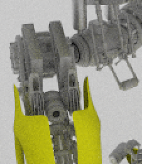
Discussion at work led to talking about implementing a wireframe shader in Nuke, so I decided to see how difficult
it would be in Imagine. As long as the mesh consists of polygons of a single type - i.e. triangles or
quads: not difficult at all it turns out.
For triangles, it’s easy enough to emulate a wireframe surface by simply working out how close a hit position
on a triangle is to an edge by transforming the triangle’s points into world space and then using the standard
point-to-line method of a perpendicular vector to each edge. This gives you the distance in world space of the
hit position to each edge, and based on which distance is the closest, you can then apply a step function to
the colour of the surface, based on the distance and a line thickness amount.
For quads, I first tried using the same algorithm as for triangles, but ignoring the edge of the triangle that was
shared within the quad. This worked to some degree, but each quad had two opposing wedges in the corners where the
point-to-line formula meant that parts of some edges weren’t shaded correctly.
So instead, I decided to use the Barycentric coordinates of the hit position within the triangle. This allowed me to correctly isolate all four edges of the quad based on a fixed threshold, but I then had to work out the line width and keep it uniform to the length of any edges. In the end I multiplied the Barycentric coordinates of both the the hit position and the inverse hit position (for the opposing edge of the quad) by the length of each of the non-shared edges of the triangle, giving a distance. The smallest of these distances I then used to step the colour, as I did for triangles. While this might not be perfectly accurate and work in all situations, it seems to work very well in practice and also allowed me to (almost) match the line thickness to the triangle method. It also looks very nice:
There’s a very slight (~1%) overhead in shading, as triangles have to be fetched and transformed to world space, but both of the renderings above at full HD finished in under six minutes with 676 samples per pixel.
When I sort out the texturing infrastructure to make it more flexible, it should be very easy to apply this texture as an alpha texture for a fully-3-dimensional mesh that is able to be seen through and cast shadows.
After recently trying to render an animation with Imagine, the result consisting of heavy aliasing in the form of walking and flickering edges on small objects, I realised that I couldn’t put off adding proper Reconstruction Filtering to Imagine any longer.
With no filtering, each sample which contributes to a pixel’s final colour has equal weighting to the final result, which leads to heavy aliasing as objects move across the frame. Using Reconstruction Filtering, the sample’s weighting to the final result is related to its distance from the centre of the pixel.
There are many different kinds of filters that can be used for Reconstruction Filtering, ranging from Box filtering (which is the same as no filtering - at least with a default filter width of 1), Gaussian (smooth, slightly blurred) to Lanczos Sinc (very sharp, having negative lobes). Unfortunately, no filter is perfect for every scenario, although generally for stills, you can get away with sharper filters.
I’ve implemented Triangle, Gaussian and Mitchell Netravali filters currently, which along with Box (no filtering) you can see enlarged examples of below:
The majority of the time spent when raytracing is generally intersecting rays with the scene and the objects in the scene. The two main ways to reduce the time taken to raytrace scenes are to either reduce the cost of each ray intersection (by using acceleration structures), or to send less rays.
Sending less rays obviously has a direct impact on the speed of rendering the scene, but care has to be taken to make sure image quality doesn’t suffer as a result: normally more samples per-pixel are used in order to reduce the noise (or variance) in an image. There are a variety of techniques that can be used to maximise the effectiveness of the rays sent out into the scene from adaptive super-sampling (sending out more rays per-pixel when the samples within the pixel are dissimilar) to efficient sampling (by ensuring that there’s a good distribution of samples across all sampling dimensions) through to importance sampling.
Importance Sampling is a technique whereby samples are selected so that a variable that has the most effect on the variance of the overall end result has the most distribution.
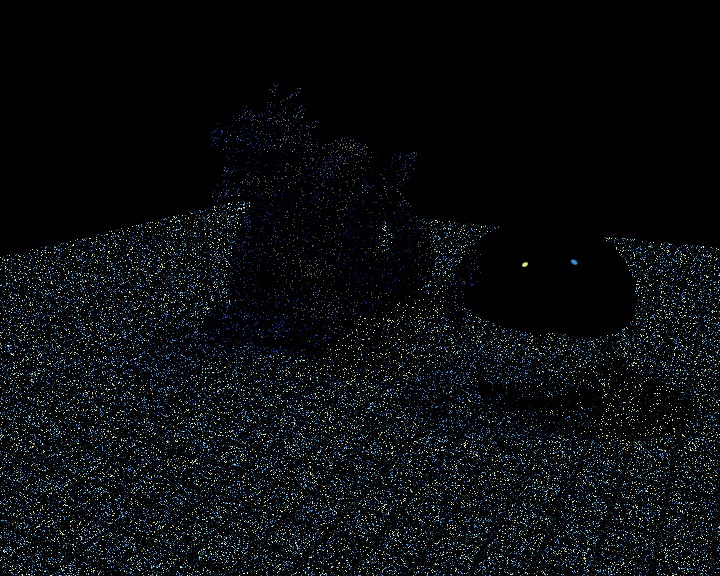
An excellent example of this is with environment lighting - if we use the following environment map for lighting a scene:
there are only two very small areas of illumination coming from the map. Without using importance sampling - by randomly sampling locations from the map - there is a low probability that any of the samples will actually correspond to the two coloured dots on the texture map. This means that either the image will be too dark (and won’t evaluate the two coloured dots correctly), or there will be very high variance where a few samples that sample the light pick up one of the coloured spots, but most don’t. This will result in extreme noise, as can be seen in this render without importance sampling:
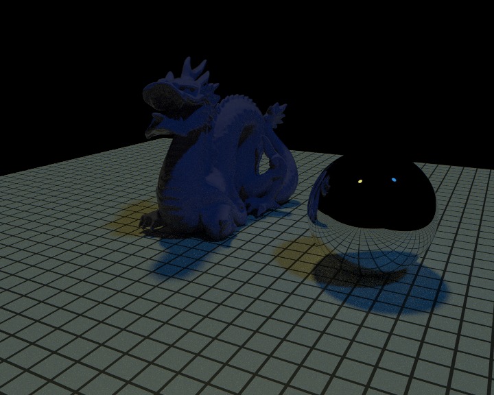
With importance sampling, it is possible to build up a two-dimensional map of importance based on the corresponding luminance of the environment map, which allows any light sample for the environment map to map to an actual position on the texture map where there is colour - i.e. one of the two coloured spots. The weighting of the function has to be modified as well, in order to not bias the equation (by assuming that the entire image is yellow and blue with no black) which would give unrealistic results.
The final result with importance sampling can be seen below:
Both images were rendered with 32 samples per-pixel, and the noise-reduction importance sampling gives in this case is striking.
The ideal situation in terms of efficiency for a raytracer when tracing rays around a scene is that the acceleration structures take the brunt of the work (assuming a simple use-case with no complex shading, displacement/subdivision or asset paging) - that is, if you profile the raytracer, the acceleration structure intersection functions are being hit more than the actual intersection functions of the primitives within the acceleration structures. This depends on quite a few things, like the layout of the scene, the acceleration structure, the geometry and how tightly boundary boxes (of either the object or any the acceleration structures use) fit around geometry or other areas.
There’s a balancing point between the density of the geometry being intersected against and how efficient the acceleration structure being used is. With a KDTree (and to a lesser extent with BVH or BIH), this is generally governed by the depth of the acceleration structures. With a Grid acceleration structure, this is done by the number of grid cells the scene area or mesh is covered by. Up to a certain point (and assuming the acceleration structure works well) increasing either of these variables increases the efficiency of the overall ray intersection process, as in ideal situations (generally most of the time), this allows less intersection tests to be needed, because the cells of the acceleration structure storing the primitives store less primitives, so less primitives have to be tested against the ray. However, increasing these numbers comes at a price - the build time of the acceleration structure goes up, as does the amount of memory required to store it. In the KDTree’s case, both of these can quite quickly become prohibitive.
Something that is common with acceleration structures (especially KDTrees, Grids and BIHs) is the fact that primitives within the acceleration structure can often be in multiple nodes or cells at once if they straddle the boundary. Due to the way most ray traversal algorithms work with the respective acceleration structures, they generally involve walking the ray through the structure until it finds nodes or cells with primitives in, and then testing each primitive in that node/cell against the ray. In the case when a ray didn’t intersect with any primitives in one node/cell and so the ray moves to the next node/cell, if some of the primitives in this next node were in the previous node as well, they will have already been intersected against the ray, so they’re not going to intersect that primitive this time. This can be quite wasteful.
In A fast voxel traversal algorithm for raytracing, J. Amanatides and A. Woo introduced a method to avoid this inefficiency, whereby each ray and each primitive have a unique ID, and when a ray is intersected against a primitive, a 2D matrix is marked with the respective ray and primitive IDs, so that a fast lookup can be done in the future to skip the test if the situation arises again. This works very nicely when there are a few number of rays (e.g. only one for physics collision tests or similar) or when there are a fairly low number of primitives and rays. But when the number of primitives and rays are both in the millions, then the amount of memory required to store this matrix becomes ridiculous, not to mention causing huge CPU cache latency problems (due to cache misses), which significantly outweigh any benefit that using the technique might provide.
In Realtime Ray Tracing on Current CPU Architectures, C. Benthin introduced (section 4.4.4) the “Hashed Mailbox”, whereby, because for a particular ray intersection test (assuming a fairly good acceleration structure) the ray will only have to be intersected against a small subset of the total number of primitives that exist, a much smaller amount of memory is actually required in order to still give a useful efficiency boost. So a small amount of memory (with around 64 slots) is allocated, and the slots to use for marking primitives that have been checked are selected based on hashing the primitive ID. This gave on average between 15% to 25% speed increases. This new technique still requires a fair amount of memory (1KB) to be allocated and freed however, which can itself still have an overhead, especially if it is done on a per-ray-intersection basis.
In Ray-triangle intersection algorithm for modern cpu architectures, A. S. Maxim Shevtsov and A. Kapustin introduced “Inverse Mailboxing”, which uses even less memory (32 bytes for an 8-mailbox slot structure), which simply stores the last eight intersected objects on the stack, and so can be easily used within the ray traversal code/algorithm. This method doesn’t guarantee that duplicate object intersection tests will not be made per-ray for any object, but assuming a decent acceleration structure and a limited number of primitives per node or cell, the chances of duplicate checks will be very small, while still providing a useful speedup.
I’ve found using this last technique has for general meshes given between 7%-23% speedups, and in the case of compound objects (objects with sub-objects within them) - where the cost of intersecting the sub-objects can be much more expensive than just a simple primitive intersection - up to a 40% speed increase.