Basic Apple M2 Pro CPU Benchmarks

This month I bought and received a new Apple MacBook Pro (M2 Pro, 14-inch, 2023) with the aim of replacing my own Apple MacBook Pro 15-inch (Intel) 2015 model which I bought in 2016. The MacBook Pro 15 still does work, but the battery life is awful now (I could have it replaced, which I’ve done several times with laptops in the past), the internal fans barely work, and the rubber around the screen is disintegrating, so with a trip back to the Northern Hemisphere planned next month, I thought it was time for a replacement.

A year ago I was provided (on loan) a work-provided MacBook Pro 14 M1 Pro (see previous benchmarks) which I’ve been using a bit, so I knew mostly what to expect in terms of performance and from the laptop in general, but I was curious to compare the performance of the M2 Pro against the M1 Pro (and the old Intel machine).

It’s not going to be a completely fair apples-to-apples comparison, as the work-provided MacBook Pro 14 M1 Pro processor is the 10-core version which has two extra performance cores than the baseline did - having eight performance cores and two efficiency cores - and the M2 Pro I’ve just bought is the baseline model - with six performance cores and four efficiency cores - but it should provide a rough indication of what performance to expect.

The Xcode / Apple Clang compiler versions are also different: My MacBook Pro 15 (Intel) is still running quite an old MacOS version, with an older compiler which I don’t want to update, and while I did install Xcode 14.3 on the 2021 MacBook Pro M1 Pro (as well as the command line tools) in order to attempt to match what I’d just installed on my new 2023 MacBook Pro M2 Pro, clang --version still shows version 13.1.6, whereas my new 2023 M2 Pro MacBook Pro shows 14.0.3 being used, so I’m not really sure what’s going on there, as Xcode -> About Xcode shows Version 14.3.1 as I’d expect on both MacBook Pro 14 machines (and both have the command line tools for that version of Xcode installed). The MacBook Pro 14s are both running MacOS Ventura 13.4.

Tests:

Copying what I did in the test last year, I’ll be using two of my apps as benchmarks: my Mint interpreter language VM (originally based off Robert Nystrom’s excellent Crafting Interpreters Lox language tutorial) but with additional functionality and performance improvements, which I’ll use to benchmark two Mint scripts as single-threaded tests, and also my Imagine pathtracing renderer, which has native SSE intrinsics support for Intel and native Neon intrinsics support for ARM, which I’ll run in both single- and multi-threaded scenarios.

Both apps will be compiled with -march=native on the Intel side and -mcpu=native on the Apple Silicon / ARM side, using the clang version on the machine in question, as well as optimisation level: -O3.

The two Mint script tests will be loop value calculation as Test 1:

var a = 1;
for (var i = 0; i < 100000000; i += 1)
{
    a = (i + i + 3 * 2 + i + 1 - 0.42) / a;
}
print a;

and a variation of Project Euler 21 to calculate the sum of all Amicable numbers under 15,000 as Test 2.

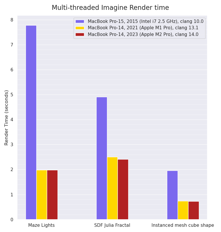
The Imagine rendering tests will render three different scenes in both single- and multi-threaded mode.

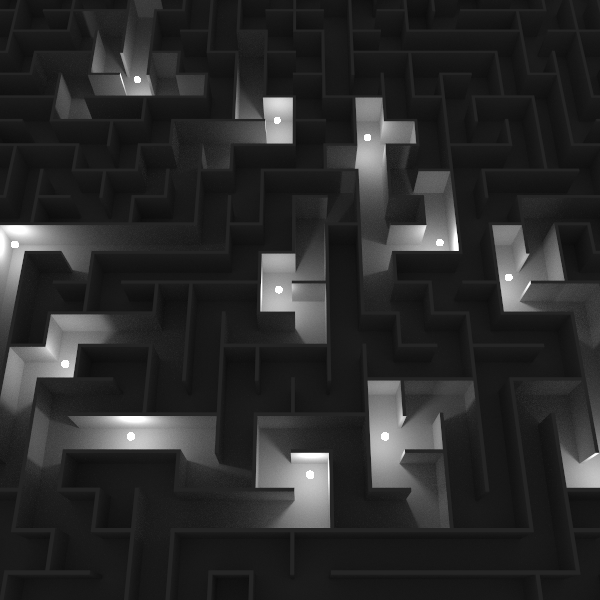
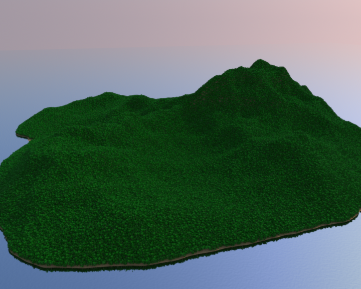
The first render will be the same maze scene with spherical area lights that I used in the test last year (example image above), but with different settings: resolution will be 256 x 256, 256 samples-per-pixel will be used, but this time only one next-event light sample will be taken each path vertex. The general ray traversal and ray intersection will utilise SIMD, but the (fairly expensive) perfect light sphere sampling is scalar, and very unlikely to be vectorised by the compilers themselves.

The second render will be a 450 x 338 resolution render of a Signed Distance Field primitive of a Julia Fractal (example image above, although with different settings), which is quite expensive to evaluate, and also does not have any SIMD utilisation for the SDF evaluation / intersection. There’s a physical Sky IBL in the scene as a light, and 144 samples-per-pixel will be used, with 3x3 Blackman Harris pixel filtering being used.

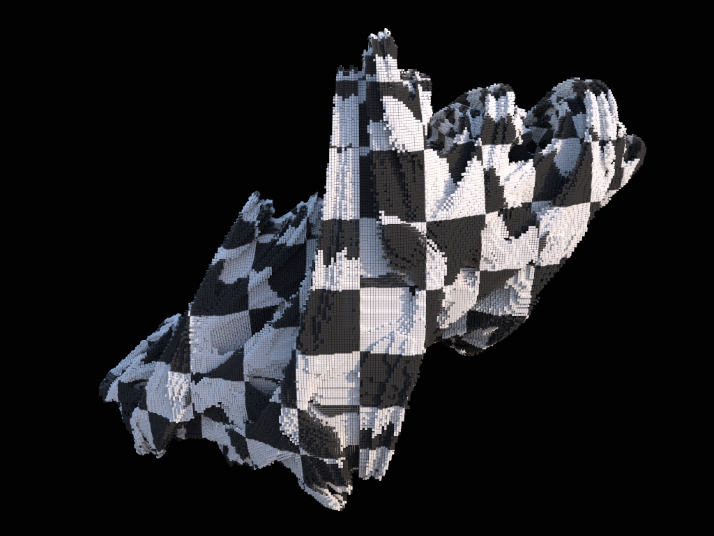
The third render will be a 450 x 338 resolution render of 2,326,299 instanced mesh cubes in the (pre-calculated) shape of a Julia Fractal, which will fully-utilise SIMD instructions for ray traversal in the BVH and for ray / primitive intersections. Again, there’s a physical Sky IBL in the scene, 144 samples-per-pixel will be used, but this time no pixel reconstruction filtering will be used (so effectively Box 1x1).

These tests will all be done on (close to fully-charged) battery power - I discovered in the tests last year that Apple doesn’t seem to down-clock on battery power - and I will also wait between test runs for the processor temperatures to be below 50 degC before running the next test, to try and reduce the impact of thermal throttling.

All tests will be run three times, and results below will show the mean average of those numbers.

Results

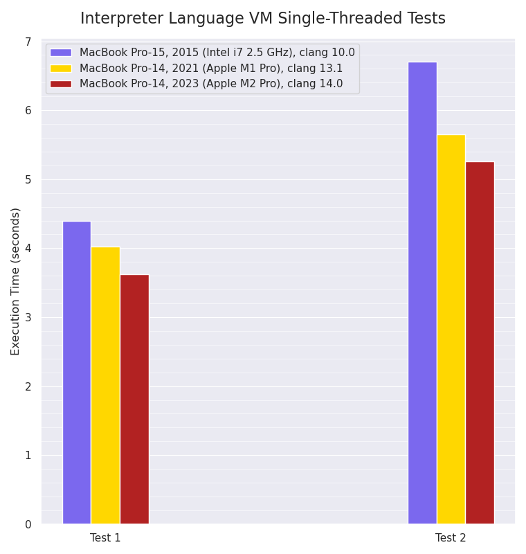
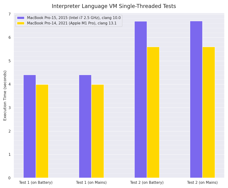
Single-threaded Mint VM interpreter:

Single-threaded Mint interpreter VM benchmarks, smaller values are better:

For these single-threaded tests, the M2 Pro has a small improvement over the M1 Pro’s performance, which itself is around 10-16% faster than the eight year old Intel i7 processor. As mentioned last year however, I think this is very likely because the Mint VM execution is often branch-prediction constrained within the main VM bytecode interpreter loop, so there’s a limit to the amount of Instruction-Level Parallelism that’s achievable from the eight-wide M1 Pro and M2 Pro.

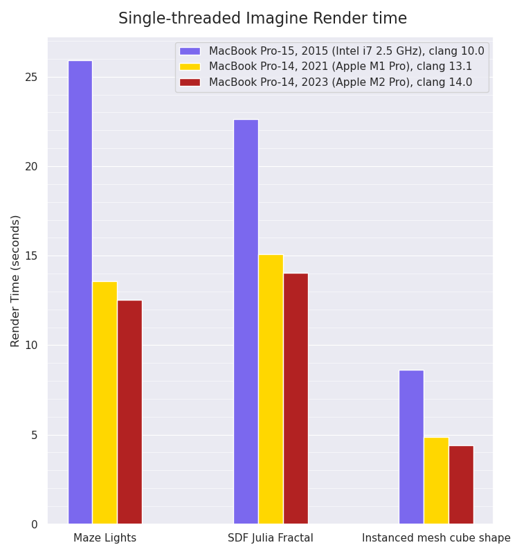
Single-threaded Imagine rendering:

Single-threaded Imagine rendering benchmarks, smaller values are better:

The single-threaded rendering tests, which have a lot more floating point calculations and SIMD usage, show a small performance improvement for the M2 Pro over the M1 Pro. Intriguingly, the Maze Lights scene is the test with the biggest performance increase (almost 2x faster) from the Intel machine to the Apple M1 Pro: the other tests show slightly smaller gains, which I wouldn’t have expected. Without further microbenchmarks of various isolated parts of those tests, it’s difficult to guess why that might be, but the different render tests do exercise different calculations and code paths.

Multi-threaded Imagine rendering:

Multi-threaded Imagine rendering benchmarks, smaller values are better:

The multi-threaded rendering tests show that due to the fact the M1 Pro machine has eight performance cores and two efficiency cores, whilst the M2 Pro machine only has six performance cores and four efficiency cores, the M2 Pro machine is only very slightly faster in the SDF Julia Fractal render scene than the M1 Pro machine, and ties in the other two tests. Once again, the Maze Lights scene shows the biggest performance increase - almost 4x faster - from the Intel CPU to the Apple Silicon ones, with the other two tests showing a less dramatic difference (between 2x to 3x faster).

Conclusion

I think a not too bad showing for the baseline model: the M2 Pro can beat the M1 Pro by a small margin in all single-threaded tests, and can either just about equal or slightly beat the M1 Pro which has more performance cores (but two less efficiency cores) in the multi-threaded tests.

Basic Apple M1 Pro CPU Benchmarks

Last week I received a work-provided (on loan) new Apple MacBook Pro (14-inch, 2021) with the Apple M1 Pro 10-core processor, so I was very curious to see how it performed with some of my code, given the generally excellent reviews and reports I’d seen by people with it online.

I have my own MacBook Pro 15-inch 2015 (Intel i7) model which I’ll be comparing it against as a basic benchmark performance test, although it won’t be a completely fair test as the two machines are running different versions of MacOS and the clang compiler, and I didn’t want to upgrade my own machine’s MacOS version to a newer version (for various reasons). So the code being executed on the different machines will be generated by different versions of clang, but given the micro-architecture is totally different anyway, I think it’s still a meaningful test and at least will show the performance difference between the two laptops.

My old MacBook Pro 15-inch 2015 is a 2.5 GHz Intel Core i7, with four cores, eight threads, and 1600 Mhz DDR3 memory, running macOS 10.14.5 (Mojave), with Xcode 10.2.1 installed which has clang version 10.0.1.

The new MacBook Pro 14-inch 2021 is the M1 Pro 10-core version, with 8 performance cores and 2 efficiency cores, running macOS 12.3 (Monterey), with Xcode 13.4.1 installed which has clang version 13.1.6.

Tests:

I’ll be using two of my apps as benchmarks: my Mint interpreter language VM (originally based off Robert Nystrom’s excellent Crafting Interpreters Lox language tutorial) but with additional functionality and performance improvements, which I’ll use to benchmark two Mint scripts as single-threaded tests, and also my Imagine pathtracing renderer, which has native SSE intrinsics support for Intel and native Neon intrinsics support for ARM, which I’ll run in both single- and multi-threaded scenarios.

Both apps will be compiled with -march=native on the Intel side and -mcpu=native on the Apple M1 Pro ARM side, using the clang version on the machine in question, as well as optimisation level: -O3.

The two Mint script tests will be loop value calculation as Test 1:

var a = 1;
for (var i = 0; i < 100000000; i += 1)
{
    a = (i + i + 3 * 2 + i + 1 - 0.42) / a;
}
print a;

and a variation of Project Euler 21 to calculate the sum of all Amicable numbers under 15,000 as Test 2.

The Imagine rendering tests will render the below example scene of a basic maze with 12 spherical area lights and one hemisphere light, with four Next Event Estimation samples being taken each bounce to evaluate the lighting, and using Cone sampling to perfectly sample each spherical area light from each hitpoint, with 256 samples-per-pixel being done, using stratified sampling and a ray depth of 6 diffuse bounces. Depending on the setup of the tests (single-threaded, multi-threaded, etc), I’ll render the scene at resolutions of: 150 x 150, 300 x 300 and 600 x 600.

For all tests, I’ll run them on battery power and then mains power, in case that affects the clocking of the processors, and will also wait between test runs for the processor temperatures to be below 50 degC before running the next test, to try and reduce the impact of thermal throttling. However, for the longer-running multi-threaded Imagine rendering tests I’m fairly sure thermal throttling will start to take place on the Intel 2015 machine given how fast the fans start to spin in longer-running scenarios.

All tests will be run three times, and results below will show the mean average of those numbers.

Results

Single-threaded Mint VM interpreter:

Single-threaded Mint interpreter VM benchmarks, smaller values are better:

For these single-threaded tests, the M1 Pro has fairly modest (~11% faster in Test 1, ~16% faster in Test 2) improvements over the seven year old Intel i7, however as the Mint VM execution is often branch-prediction constrained within the main VM bytecode interpreter loop, I expect this doesn’t really allow the M1 Pro’s eight-wide design to really stretch its legs running these benchmarks, as there’s a limit to the amount of Instruction-Level Parallelism that’s achievable.

It’s interesting to see that there’s no apparent difference in performance between running on battery vs running connected to the mains: I was expecting to see a difference - even if only on the Intel i7 MBP - as I know my Thinkpad T480s running Linux shows significant performance differences between the two states, but Apple clearly don’t seem to be implementing that strategy.

Single-threaded Imagine rendering:

Single-threaded Imagine rendering benchmarks, smaller values are better:

Things start to look more impressive for the M1 Pro in the single-threaded rendering tests, as here there are a lot more floating point calculations being done with a lot less branching, and there’s a fair amount of SIMD use (i.e. ray intersection / traversal code, which uses native SSE or Neon instructions for the respective platform architectures) allowing the M1 Pro to show what it can do.

For both the 150 x 150 resolution and 300 x 300 resolution renders, the M1 Pro machine completed the tasks in ~46% less time, so it’s close to twice as fast as the older Intel machine. Again, there was no apparent performance difference between running powered off the battery compared to running with the machines plugged into the mains power.

Multi-threaded Imagine rendering:

Multi-threaded Imagine rendering benchmarks, smaller values are better:

The multi-threaded rendering tests show that for the shorter-duration 300 x 300 resolution render, the M1 Pro was more than three times faster (render time was less than a 1/3 of the Intel MBP’s i7 render time), and for the longer-duration 600 x 600 resolution render this ratio was slightly better still - I suspect because of the fact the Apple M1 Pro has significantly better thermal performance than the Intel i7, so is not throttling as much - if at all - although watching the temps on the M1 Pro machine towards the end of the test shows it did reach 84 degC, so it’s possible throttling is happening a bit.

Conclusion

So for most code that’s likely not branch/dependency-bound, it would seem the almost one year-old M1 Pro being tested here is around three times faster than the seven year-old Intel i7 model (although the base M1 Pro model with two less performance cores will not be as fast), and for multi-threaded code that parallelises well it can be more than three times faster, with much better thermal performance (which means less fan noise) and battery life, which is exactly what you’d want from a laptop, and I think shows that the Apple M1 processors are something to be excited about.

Interpreter Programming Language Benchmarks

I’ve sporadically but progressively been continuing to work on my Mint interpreter programming language/VM that was heavily based off Robert Nystrom’s excellent Crafting Interpreters Lox language tutorial, and have spent a fair bit of time trying to optimise the main VM bytecode despatch loop among other areas of the VM, as well as performing some benchmark comparisons with other similar bytecode VM interpreter languages like Lua, Python and Ruby to see where Mint stands performance-wise as well as to understand how fast the other VMs are, how they work and some of their performance characteristics for different things.

I managed to speed up the original HashMap implementation a bit by caching the capacity mod bit-mask and the capacity and table load ratio, so as to not recalculate them on-the-fly every lookup which wasn’t needed, and to only update them when the table resized, in addition to adding some compiler hints in order to force inline things and give hints on branch prediction likelihood which helped a bit more.

One of the main bottlenecks in raw execution speed is the main VM stack in terms of operations pushing and popping items onto and off it, so this is really the hot loop of the VM - at least when the Garbage Collector is not being exercised. On the bytecode opcode execution side of things, I added some new opcodes in order to do some things more efficiently, for example to operate directly on items within the stack in certain limited scenarios when constant values are used, without having to pop and push them back - for example this can be used by compound assignment operators like +=, -=, *=, etc, with constant values being used as the right-hand-side argument, and helped speed things up a bit.

For general for loops incrementing a value by 1 each time, the push/pop overhead was fairly substantial, and I added a dedicated OP_INC_LOCAL opcode to help with this, which can increment the top of the stack by one without popping the stack and then having to push the result after adding 1. The compiler part can detect when this can be used (e.g. in the for loop increment clause, with a constant value being used as the increment) and will use it when possible.

Lua - being a register-based interpreter VM - seems to have an advantage in the area of performance - especially in maths-heavy code - because it doesn’t need to do as many stack operations, and this is one of the reasons Lua is one of the faster bytecode interpreter languages.

The main dispatch loop can also be optimised by using “computed gotos” instead of just a case statement for each opcode within a switch statement: with switch / case statements, compilers are obliged (in C and C++ anyway) to add an upper bound value check, which slows down execution.

In terms of where things stand now performance-wise, I’m fairly happy: Mint is not the fastest interpreter language VM, but it is very competitive against Python 2, Python 3 and Ruby in most cases, and occasionally can win against Lua.

For performance comparisons, I’ve mostly been using basic problem solving exercises from Project Euler which are normally maths-heavy, meaning the benchmark test programs I’m using are slightly skewed benchmarks towards maths operations compared to more general operations (i.e. they don’t generally exercise the Garbage Collector infrastructure), but that’s the type of code execution I’m mostly interested in for the moment.

I’m going to compare Mint against four (I’ll compare Python 2 and Python 3 separately) other interpreter language VMs:

• Lua 5.3
• Python 2.7
• Python 3.8
• Ruby 2.7

These are the package versions available with the Linux distro I’m using (Linux Mint) on my laptop, and I’m going to compare them against Mint (VM) built with GCC 9.3, as that’s the system compiler version that I assume the packages for the other interpreter language VMs were compiled with, so seems the fairest compiler to use to compile with. Mint will be built with optimisation level -O3. Normally I like also comparing different compiler versions and optimisation levels, but I’m not going to do that this time as my aim is to compare against other interpreter VMs, and that would increase the number of tests I’d have to do quite a lot, and I’d rather not get into building each one from source, but that would be the fairest way of doing a fully-comprehensive comparison if I had the time.

The tests are being done on a laptop with an Intel i5-8350U processor, with the power plugged in. I’ll make sure the CPU temp is normal before running each test to prevent thermal throttling, and will run five identical tests of each benchmark with each interpreter language, using the mean average as the final result.

I will run the following seven tests:

As quick partial examples, here is the Mint script code for Test 3:

var a = 1;
for (var i = 0; i < 100000000; i += 1)
{
    a = (i + i + 3 * 2 + i + 1 - 0.42) / a;
}
print a;

here is the Lua version of Test 3:

local a = 1
for i = 0,100000000-1
do
    a = (i + i + 3 * 2 + i + 1 - 0.42) / a;
end
print (a)

here is the Python 3 version:

a = 1
for i in range(0, 100000000):
    a = (i + i + 3 * 2 + i + 1 - 0.42) / a
print(a)

and here is the Ruby version:

a = 1
0.upto 100000000-1 do |i|
    a = (i + i + 3 * 2 + i + 1 - 0.42) / a
end
print a
print "\n"

These are the results, showing average execution time for each test for all interpreter language VMs (smaller values are better):

Lua has a very good showing (largely I think because it’s a register-based VM instead of a stack-based one), and I’d expect the non-JIT version of LuaJIT which is heavily-optimised on x86-x64 would be even faster.

Mint just wins in Tests 6 and 7, and is second fastest in the remaining tests, which isn’t bad as far as I’m concerned. There’s more room for optimisation - especially with regards to the Garbage Collector which these benchmark tests purposefully didn’t exercise, but also in other areas, i.e. Constant Folding is on my list to look at implementing - but I’m happy enough with the improvements and speed for the moment.

PRNG Evaluation and Benchmarks for Monte Carlo Simulations

Imagine - being a stochastic pathtracing renderer, utilising the Monte Carlo method of random sampling to solve the Light Transport Equation - has had the need to generate large quantities of random numbers since fairly early on in its life, when I added support for Ambient Occlusion at the time it was still doing Whitted Raytracing (before I implemented full pathtracing support later that year). Initially, I was naively using the system rand() call to generate unit interval floating point values, like so:

float randomFloat()
{
	return rand() / (float(RAND_MAX) + 1.0f);
}

however I quickly realised this was incredibly slow due to all the system calls (especially on OS X, which I was mostly using at the time for development - on Linux the system call overhead was not as bad), as well as providing duplicate results between multiple threads (there’s a _r-suffix version for that problem). Around the same time I had just started reading PBRT 2, which had a basic version of the Mersenne Twister which I implemented, and got significant speed-ups from using instead. A few months later, I discovered the existence of the SIMD-oriented Fast Mersenne Twister version, which used SSE intrinsics instructions to speed up generation, which provided a bit of an extra boost.

Since then, I haven’t really thought that much about the PRNG (Pseudo-Random Number Generator) within Imagine in terms of speed (or quality), partly because sample generation wasn’t generally that much of an overhead (although in some pathological cases it could be more noticeable, i.e. non-adaptive renders doing large numbers of samples per pixel with almost nothing in the scene would end up spending a fairly large proportion of the CPU time generating samples), but also because Imagine uses several techniques to make sure the samples it uses based off the generated random numbers are well distributed amongst dimensions, and there was a tiny bit of leeway in how good the samples needed to be due to this (although better ones would still be more ideal). On top of that, I’d more recently implemented support for Low Discrepancy Sequences - like the Halton sequence - which are an alternative method of generating series of quasi/pseudo random numbers, and have some advantages in terms of being able to progressively draw samples with very low overheads that are well distributed/de-correlated with the samples from previous sequences, meaning the PRNG infrastructure wasn’t always being used as much.

I had become aware that the Mersenne Twister was far from state-of-the-art these days, and that there were much faster non-secure PRNGs available, often with better statistical properties as well, and I recently was curious to investigate some of them from a performance perspective, but also to do some fairly primitive - and unlikely to be statistically-principled! - evaluations of some of the results generated from them in the context of using them to generate the types of numbers Imagine requires for Monte Carlo sampling, which are essentially:

• 32-bit floating point unit interval numbers (between 0.0 and 1.0)
• 32-bit unsigned integers.

The basic statistical analysis I did of the generated random numbers was partly to see if I could notice any obvious issues, but mostly to ensure that my implementations and use of them were correct, and didn’t have any obvious bias or clumping issues in the distributions.

There are several fairly recent comparisons of PRNGs online which both benchmark them and provide some analysis of output from random number statistical analysis packages like PractRand, but they mostly seem to concern themselves with 64-bit integer numbers and double-precision floating point numbers which may or may not be directly relevant to the lesser requirements Imagine has. On top of that, some of the comparisons are using older PRNGs like Xoroshiro128 when there are newer versions like Xoshiro256 with apparently better properties (depending on which variant is used).

With that in mind, I decided to compare the following PRNGs:

• Linux System rand48()/drand48() calls
• Original Mersenne Twister (MT19937)
• SFMT (SIMD oriented Fast Mersenne Twister)
• Lehmer LCG
• PCG32
• Xoshiro256+
• Xoshiro256++

I’m including the System rand48()/drand48() simply an an interesting baseline, and several of the other choices (Lehmer LCG, and the two Mersenne Twister variants in particular) technically have some statistical issues with regards to quality, but I’m curious if I can actually spot any biases / issues in some of the basic evaluations I’ll be doing. It should be noted that some of these PRNGs do generate 64-bit numbers (the Xoshiro256 versions for example), but while I will use the code to generate those numbers, I will only be using float32 and uint32_t numbers. The other PRNGs (the two Mersenne Twisters, PCG32 and the LCG return 32-bit numbers, although PCG32 has the ability to generate 64-bit numbers, but I’m not using that).

PCG32 and the two Xoshiro256 variant PRNGs will be seeded using the SplitMix64 algorithm (which in itself is a PRNG of sorts), doing 16 shuffle rounds using SplitMax64 from the original single 32-bit seed number, and then using the required number of uint32_t values from the SplitMix64 generator for the state the PRNG needs.

I’m going to do several variations of the same type of tests, which will be very basic attempts to evaluate the distribution / uniform-ness of the random numbers. There are various statistical ways to do this in a more principled way (Chi Square test, Kolmogorov-Smirnov test, etc), however those aren’t perfect methods themselves, and I’d prefer something more visual, even if it is less principled and less robust. With that in mind, I’m going to generate binned “histograms” or density charts of number ranges and sample size combinations, and plot them in image form, in other words having a single pixel representing a histogram bin, and the colour of the pixel representing the value, with darker pixel values meaning the density of samples in that bin were higher.

All PRNGs for each same test will be seeded with the same source random number, however the different PRNGs will internally handle state initialisation from this seed in the recommended way (i.e. SplitMax64 in some cases), but each test type will use a different seed number.

1D floating point number generation

The first set of evaluation tests will be drawing a series of independent floating point numbers between 0.0 and 1.0, and converting that floating point number to an integer “histogram” bin index, and then incrementing the bin count for that bin index. After fitting these random number results into bins, the bin counts will then be normalised to the bin count with the maximum count, and a strip width PNG image with vertical bars of fixed strip height representing the normalised bin count density will be written out, with darker bars meaning higher bin counts. The test series will use 500 histogram bins (and so the image width will be 500 pixels, each horizontal pixel representing one histogram bin), and different densities of random numbers will be drawn for each series:

1. 500 - low density to match the bin count
2. 50,000 - a medium density of samples
3. 5,000,000 - a high density of samples.

The average sum of these random numbers will also be recorded for each test (total sum of all 0.0 -> 1.0 random numbers drawn, divided by the number of random numbers drawn), which should average out to as close to 0.5 as possible.

Low Density 1D 500 Bin Histogram:

Results with 500 samples:

PRNG	500 bin histogram	Average
drand48()		0.523126
Mersenne Twister		0.495327
SFMT		0.481424
Lehmer LCG		0.488260
PCG32		0.507498
Xoshiro256+		0.501831
Xoshiro256++		0.513263

This test run is pretty unfair, as there’s only 500 random numbers that need to fit into 500 bins, so even with an extremely good PRNG there will be some clumping, and that’s going to be somewhat dependent on the bin widths (1.0 / 500 in this case). It would also likely be a bit fairer to do multiple runs with different seed numbers to show variations, but I haven’t really got time for such a comprehensive investigation as that, this is really just a representative look at a general sampling of the numbers to check for any obvious issues in the number distributions of my implementations.

It’s difficult to really draw any conclusions from this single test, but it might be possible to argue that the drand48() test shows the most clumping of values with four very dense bins, two of which are double-width adjacent bins, while Mersenne Twister, Lehmer LCG and PCG32 might seem to have the “best” distribution in this case.

Medium Density 1D 500 Bin Histogram:

Results with 50,000 samples:

PRNG	500 bin histogram	Average
drand48()		0.498131
Mersenne Twister		0.497892
SFMT		0.497343
Lehmer LCG		0.498952
PCG32		0.499932
Xoshiro256+		0.501509
Xoshiro256++		0.499024

With many more samples per potential bin, the results are much more uniform now, as the darker images show, with the average number results converging more closely to 0.5.

High Density 1D 500 Bin Histogram:

Results with 5,000,000 samples:

PRNG	500 bin histogram	Average
drand48()		0.500111
Mersenne Twister		0.500030
SFMT		0.499919
Lehmer LCG		0.500040
PCG32		0.499940
Xoshiro256+		0.500205
Xoshiro256++		0.499983

The images are too dark now to really see well, showing they’re now much more uniform (all bins are normalised to the maximum bin count). There’s still a bit of clumping, but it’s difficult to really know if this is a problem or not by just these image histograms alone. The Average number results once more converge even more closely to 0.5.

2D floating point number generation

The next set of evaluation tests will draw pairs of floating point numbers from each PRNG, and use them as X and Y coordinates to map them to a 2D histogram of 500 bins for each dimension, represented in image form by a 500x500 pixel image, with pixel values being normalised to the maximum bin count. Different densities of coordinate pairs will be drawn for each set of tests:

1. 250,000 - low density of samples to match the total bin count
2. 250,000,000 - a high density of samples.

The hope with this 2D test is to check for independence between the two numbers picked for each sample, and that there’s no correlation which shows up when using the two consecutively-generated numbers for two different dimensions.

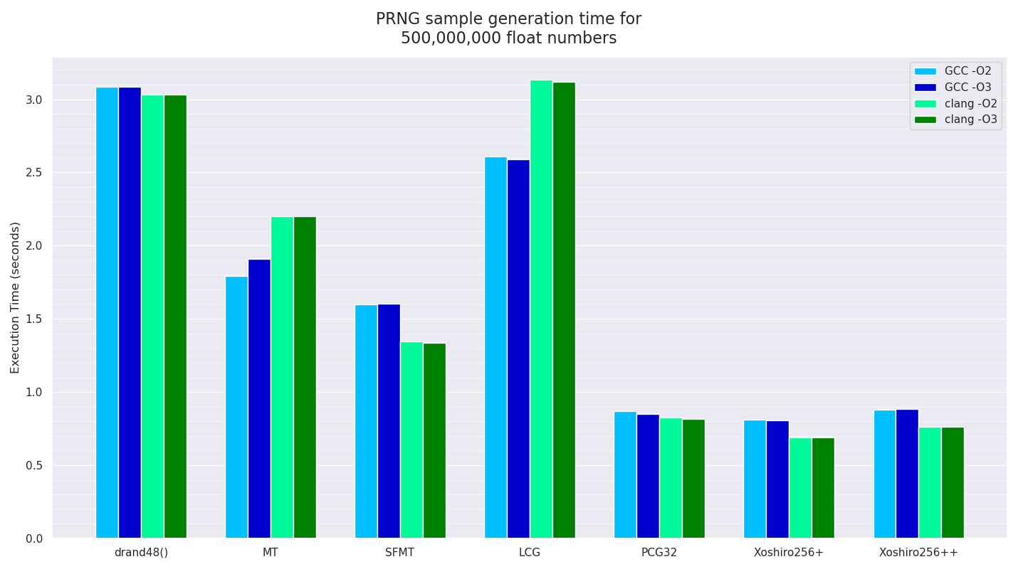
For the second high-density test of 250 million 2D samples, I will also additionally modify the code to just generate the random number float values (500 million of them) without sorting them into bins or anything else, other than accumulating the total value (to stop the compiler optimising things away) and timing how long that takes. I will test this execution time code with two compilers, GCC 9 and clang 10 on a Linux laptop with an Intel i5-8350U CPU, with the laptop plugged into the mains and ensuring the machine is idle and the CPU temp is not throttling, with both -O2 and -O3 optimised build flags with each compiler.

Low Density 2D 500x500 Bin Histogram:

Results with 250,000 2D samples:

PRNG	500 bin histogram	AverageX AverageY
drand48()		0.500969 0.499713
Mersenne Twister		0.501777 0.498884
SFMT		0.499758 0.499488
Lehmer LCG		0.498797 0.498904
PCG32		0.500417 0.499793
Xoshiro256+		0.500171 0.499525
Xoshiro256++		0.500250 0.499567

While there are different noise patterns here, there doesn’t appear to be any obvious practical difference between the different PRNGs in the above images their output generated, nor are there any obvious clumping or gaps.

High Density 2D 500x500 Bin Histogram:

Results with 250,000,000 2D samples (500,000,000 float numbers in total):

PRNG	500 bin histogram
drand48()
Mersenne Twister
SFMT
Lehmer LCG
PCG32
Xoshiro256+
Xoshiro256++

With the higher density of samples, again, there’s nothing that really stands out: it does appear that there might be extremely faint clusters of slightly darker “shapes” in the noise in the PCG32 and Xoshiro256++ images near the centre, but without further investigation, those could well just be seed-specific, so I don’t think it’s anything to worry about.

And here are the isolated mean average performance numbers of four duplicate runs for all the PRNGs to generate the above 2D samples, for both GCC and clang compilers with two sets of optimisation levels for each, running in just one single-threaded process:

The system drand48() “PRNG” was pretty much the slowest (although the LGC PRNG compiled with clang was actually slower), with LGC compiled with GCC being the next fastest. The two Mersenne Twister variants are next fastest, but as expected, no longer competitive for this use-case, with PCG32 and the two Xoshiro256 variants being the fastest, depending on which compiler was used, with Xoshiro256+ being the absolute fastest.

1D unsigned integer number generation

These tests are similar to the 1D floating point tests, however I’m natively generating unsigned int values from the PRNGs rather than converting the native integer into a float32, and am using upper-bound rejection sampling to constrain the upper limit of the unsigned int values to prevent modulo bias, so as to generate sample integer values between 0 and 499 inclusive.

These values are then mapped to the corresponding histogram bins and accumulated per bin, and at the end of generating all the random numbers, the bin count values are all normalised to the maximum bin count, and PNG images are generated, with vertical pixel bars representing each bin being drawn, with darker bars meaning more dense samples for that number.

Low Density 1D 500 Bin Histogram:

Results with 500 samples:

PRNG	500 bin histogram	Average
rand48()		249
Mersenne Twister		251
SFMT		234
Lehmer LCG		242
PCG32		235
Xoshiro256+		244
Xoshiro256++		250

With a low density of samples, it’s difficult to really see any obvious issues from the sparseness of the results, although some PRNGs do seem to produce results which are more uniform and distributed than others, although that could just be due to the particular seed value used, so more analysis would need to be done to come to that conclusion.

Medium Density 1D 500 Bin Histogram:

Results with 50,000 samples:

PRNG	500 bin histogram	Average
rand48()		249
Mersenne Twister		249
SFMT		249
Lehmer LCG		249
PCG32		249
Xoshiro256+		249
Xoshiro256++		249

With the medium density of unsigned integer samples, uniform-ness of the results is much better as expected, however Xoshiro256+ does seem to show a bit more clumping (especially at the end of the range), and Xoshiro256++ might possibly be showing a bit of clumping in the middle of the range - but again, this might be due to the particular seed value used, and using another seed value might produce different results.

As a test of this theory, here’s a duplicate set of results, but with a different initial seed value, which does seem to indicate that might be the case:

PRNG	500 bin histogram	Average
rand48()		249
Mersenne Twister		249
SFMT		249
Lehmer LCG		249
PCG32		249
Xoshiro256+		250
Xoshiro256++		249

This does appear to show that the seed value does have significant influence on any subtle clumping or patterns in these basic image representations, and a much more comprehensive and in-depth analysis would be required in order to find out and investigate for certain.

1D biased unsigned integer number generation

I then decided to see if my “histogram” tests were actually capable of detecting any modulo bias, so ran the same tests again but with the code modified to just mod a single unsigned integer number by the 500 upper limit, which is a biased way of constraining the resultant integer values, but is faster to generate.

Low Density 1D 500 Bin Histogram:

Results with 500 samples:

PRNG	500 bin histogram - biased	Average
rand48()		229
Mersenne Twister		232
SFMT		246
Lehmer LCG		229
PCG32		253
Xoshiro256+		245
Xoshiro256++		246

With biased unsigned int range-limited generated numbers with low density, there’s slightly more obvious clumping occurring now, along with some evidence of very small numbers being picked more often for many of the PRNGs, and the “average” resultant value numbers are a bit more varied and generally a bit lower than with the non-biased modulo limiting method.

Medium Density 1D 500 Bin Histogram:

Results with 50,000 samples:

PRNG	500 bin histogram - biased	Average
rand48()		245
Mersenne Twister		243
SFMT		245
Lehmer LCG		244
PCG32		244
Xoshiro256+		243
Xoshiro256++		243

Moving on to the medium density of random numbers, it now becomes abundantly clear that using a biased method of clamping the random numbers is picking very low numbers much more often than other numbers in the total required range, and that the distribution is not uniform with this method. The “average” resultant values are also now consistently lower (243-245) than the corresponding correct and non-biased version of this test above, which produced the expected average of 249 consistently for all PRNGs.

Conclusion

Based on this basic analysis / benchmark, as well as looking at what other people have decided online with their comparisons and analysis, it seems clear that Mersenne Twister / SFMT is not the PRNG to be using these days, even if purely from a performance perspective. It does also suffer from some theoretical statistical issues that more modern statistical test frameworks are capable of looking for, however it’s not clear if those are actually noticeable in practice for Imagine’s use-case of random numbers: my basic analysis above doesn’t really highlight any concerns, but there could be something very subtle there that these basic tests won’t show.

The three fastest PRNGs in these tests are PCG32, Xoshiro256+ and Xoshiro256++, and while Xoshiro256+ is the fastest, it does have some slight statistical issues with unsigned integer number generation which for some use-cases might not be ideal, and consensus seems to be that Xoshiro256++ is the safer bet, even if it is slightly slower.

So with that in mind, that’s what I’ve converted Imagine to use, and the resulting speed-ups of going from SFMT to Xoshiro256++ are fairly modest in most cases, but measurable non-the-less.

C++ Compiler Benchmarks v2

This is another comparison of C++ compiler benchmarks on Linux using my Imagine renderer as the benchmark, almost three years since I did the last set of benchmarks.

This time, I’m only comparing versions of GCC and Clang, but I am also comparing the -Os optimisation level in addition to -O2 and -O3.

As with the previous benchmarks I did, I’m sticking with just comparing the standard “stock” optimisation levels, as it’s generally the starting point for compiler flags, and it makes things a fair bit easier, rather than trying every single combination of flags different compilers can support.

As it stands now, Imagine consists of 143,682 lines of C++ in 458 implementation files (.cpp), and 68,937 lines of C++ in 579 header files, for a total of 212,619 lines of code.

The compilers that I’m comparing are:

• GCC 4.8.5
• GCC 4.9.3
• GCC 5.4
• GCC 6.3
• GCC 7.1
• Clang 3.8
• Clang 3.9
• Clang 4.0
• Clang 5.0

GCC 4.8.5, GCC 5.4 and Clang 3.8 were Ubuntu packages, the other versions I compiled from source, using the methods recommended in the respective documentation.

The machine the tests were run on is the same machine the previous benchmarks were run on, but it now has an SSD system disk (which I ran the tests on in terms of target compilation), and a more up-to-date Linux distribution (Ubuntu 16.04 LTS). The machine is a dual socket Intel Xeon E5-2643 (3.3 Ghz) of Sandy Bridge vintage. Imagine’s code has also changed quite a bit in key areas, so these tests can’t be directly compared to the previous tests.

This time I didn’t run any microbenchmarks, just three different renders of different things in Imagine, basically rendering three different scenes. Due to the amount of things Imagine will be doing (ray tracing, light transport, material evaluation, splatting, etc, etc) this does mean that there’s a fair chance that code generated for different aspects can’t really be identified, as the timing will be for the render as a whole, but I think it still provides some indication as to what the compilers are doing relative to each other.

The compiler flags used to build Imagine were:

[main test optimisation flag] -fPIC -ffast-math -mfpmath=sse -msse -msse2 -msse3 -mssse3 -msse4

Compilation Benchmarks

Compilation time:

First of all I compared compilation time of all the compilers, building all of Imagine using different numbers of jobs (threads), from 16 (the total number of logical cores / threads my machine supports), down to 2. This was to try and isolate how parallel compilation can be (in particular with hyperthreading) when disk IO is a factor. Imagine’s source code was on an SSD, as was the directory for compiling.

Three runs from clean were done with each combination, and the time was timed with the command line ‘time’ command in front of the ‘make -jx’ command.

The graph below shows the results (mean averages).

As can be seen, there’s a fairly obvious pattern of O3 builds taking slightly longer than O2 builds, and Os builds taking slightly less than O2 builds as one would expect. In GCC, going from 8 to 16 threads (so effectively using hyperthreading on the machine, although it’s not clear what the scheduler was doing) gave practically no benefit in the older GCC versions, with a possible tiny benefit with 6.3 and 7.1, although 6.3 and 7.1 take noticeably longer to compile than older versions. Thread scalability after that is relatively close to linear, the difference probably being link time which cannot be parallelised as much.

Clang is consistently slower than GCC to build. I saw this in my previous tests I ran almost three years ago, and while in those tests I incorrectly enabled asserts when building it from source, making Clang builds slightly slower, even when disabling asserts back then it was still slower than GCC. This time I made sure asserts weren’t enabled, and it still seems to be slower than GCC, which seems to be against conventional wisdom, however it seems pretty consistent here. 5/6 years ago, I definitely found Clang faster to compile than GCC (4.2/4.4) when I benchmarked it, but that no longer seems to be the case.

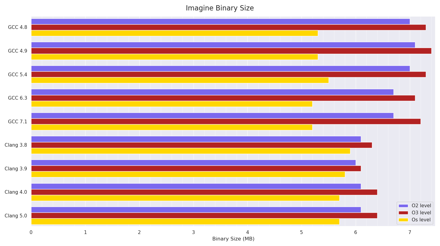
Executable Size:

Below is a graph of the resultant executable size:

The pattern of O3 builds being bigger than O2 builds due to more aggressive optimisations (probably mainly more inlining and loop unrolling) is visible, and it’s noticeable how much smaller than O2 builds GCC’s Os builds are compared to Clang’s.

Rendering benchmarks

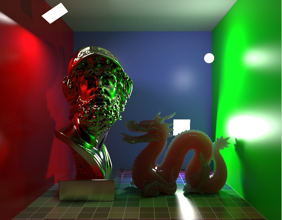
Scene 1:

Scene 1 consisted of a Cornell box (floor diffuse procedural texture with Beckmann microfacet spec lobe, walls diffuse + Beckmann microfacet spec lobes), with one bust model consisting of 544k triangles with a conductor microfacet BSDF (GGX), a dragon model consisting of 535k triangles with dielectric refractive lobe with brute force internal scattering for SSS with multiple scattering, and Beckmann microfacet dielectric lobe.

Three area lights (two quads, one sphere) were in the scene, each of which was sampled per hit / scatter (for next event estimation).

The resolution was 1024x768, with max path length of 6, using a volumetric integrator (which calculates full transmission for shadows, so it can’t early out in most cases), in non-progressive mode, using 144 stratified samples per pixel in basic pathtracing mode (no splitting) with MIS. The Mitchell-Netravali pixel filter was used for splatting.

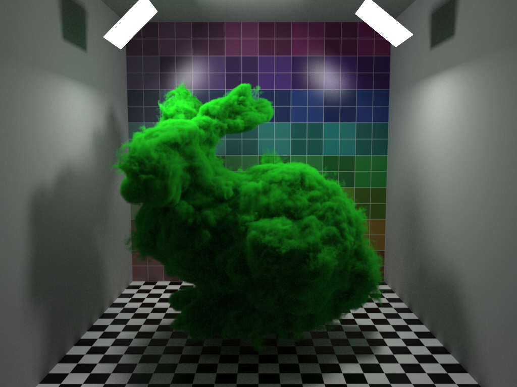
Scene 2:

Scene 2 again consisted of a Cornell box, but with more basic materials (only the back wall had a spec lobe on in addition to diffuse), with two quad area lights, and a dense voxel grid volumetric bunny (converted from OpenVDB examples) with an Isotropic phase function. The resolution was again 1024x768, with max path length of 6, with 81 stratified samples used in non-progressive mode. The volumetric integrator was used, with Woodcock tracking volume sampling for the heterogenous voxel volume, with multiple scattering, and two transmittance samples per volume scatter event per light sample. Both lights were sampled per surface and volume scatter event for next event estimation. Volume roughening (falling back to nearest neighbour voxel lookup after ray roughness / throughput reaches a threshold) was turned off, so full trilinear voxel lookups were always done.

Scene 3:

Scene 3 consisted of a single 10M triangle mesh of a scanned church ornament, with a diffuse texture provided by a 1M point pointcloud lookup texture (KDTree). A very large filter radius was needed on the point lookups, due to the weird arrangements of the colour point values in the pointcloud in order to not have gaps in the resulting texture. A constant Beckmann spec lobe was also on the material.

A single Physical Sky Environment light was in the scene, with Environment Directional culling (culling directions on the Environment light that aren’t actually visible from the surface normal) disabled.

The resolution was 1024x768, max path length was 5, and a non-volumetric integrator was used this time, meaning occlusion ray traversal could early-out instead of having to find the closest hit and test transmittance through materials as the volume tests above had to. 81 stratified samples per pixel were used in non-progressive mode, with MIS path tracing.

Performance Results

Six runs of each were done, restarting each time to account for possible different memory layouts - Imagine is NUMA aware where possible, trying very hard to allocate and write (first touch) memory dedicated to the core/socket that will be running, but some things like triangles / geometry / acceleration structures can’t really be made NUMA-aware without duplicating memory which doesn’t really make sense, so it’s somewhat down to luck where memory will be (in terms of attached to which socket). 16 threads were used for rendering, and render thread affinity was set. The times are in seconds, and are for pure rendering (no loading, scene building or acceleration structure building included in the times), and were measured with code within Imagine. Mean averages are graphed below.

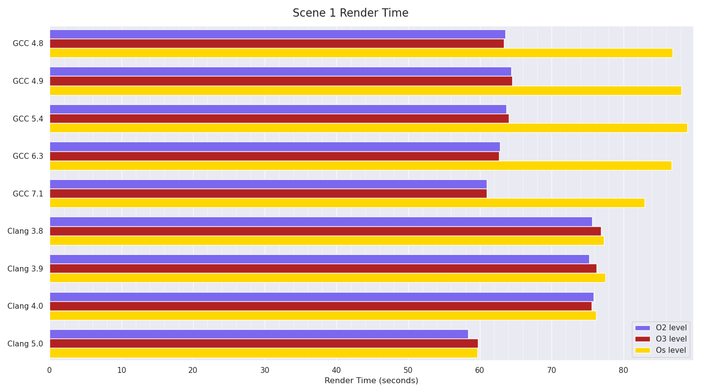
Scene 1

Scene 1 results show GCC 7.1 made some improvements over previous GCC versions, and that GCC’s Os builds are noticeably slower than its O2 or O3 ones. Until Clang 5.0, Clang was noticeably slower than GCC, however Clang 5.0 managed to just beat GCC 7.1’s numbers. Interestingly, Clang’s Os numbers show almost no difference to its more optimised builds, in contrast to GCC’s ratio between the optimisation levels.

Scene 2

Scene 2 shows a regression in performance going from GCC 4.9 to 5.4, which still hasn’t been recovered in GCC 7.1. Clang wins these by a comfortable margin. Again, Clang’s consistency between different optimisation levels is very close, in contrast to GCC’s, which is more pronounced.

Scene 3

Scene 3 is fairly similar to Scene 1 in that GCC 7.1 makes slight gains over previous GCC versions (and is the fastest), while until Clang 5.0, Clang was noticeably slower than GCC. Clang 5.0 almost makes up the gap to GCC 7.1.

Conclusion

Given these benchmarks are pretty much “overall” benchmarks, given within each test Imagine is doing so many different things, it’s very likely things are averaging out between the compilers, however, it does seem that Clang 5.0 made significant improvements over Clang 4.0 in two of the tests, becoming the new fastest in Scene 1 and almost matching GCC 7.1 in Scene 3. GCC 7.1 is the fastest in Scene 3, and almost the fastest in Scene 1, but GCC’s speed regression from 4.9 -> 5.4 in Scene 2 still impacts GCC 7.1, meaning Clang completely dominated Scene 2.

What was very interesting to me was the speed penalty GCC’s Os builds have compared to Clang’s Os builds. Given the executable size graph shows a similar ratio in terms of GCC’s Os builds being noticeably smaller than GCC’s O2 builds than Clang’s Os builds are than Clang’s O2 builds, it seems fairly obvious from the executable sizes produced that Clang is still fairly aggressively optimising Os builds, in contrast to GCC which seems to much more strongly prioritise smaller executable size.

C++ Compiler Benchmarks

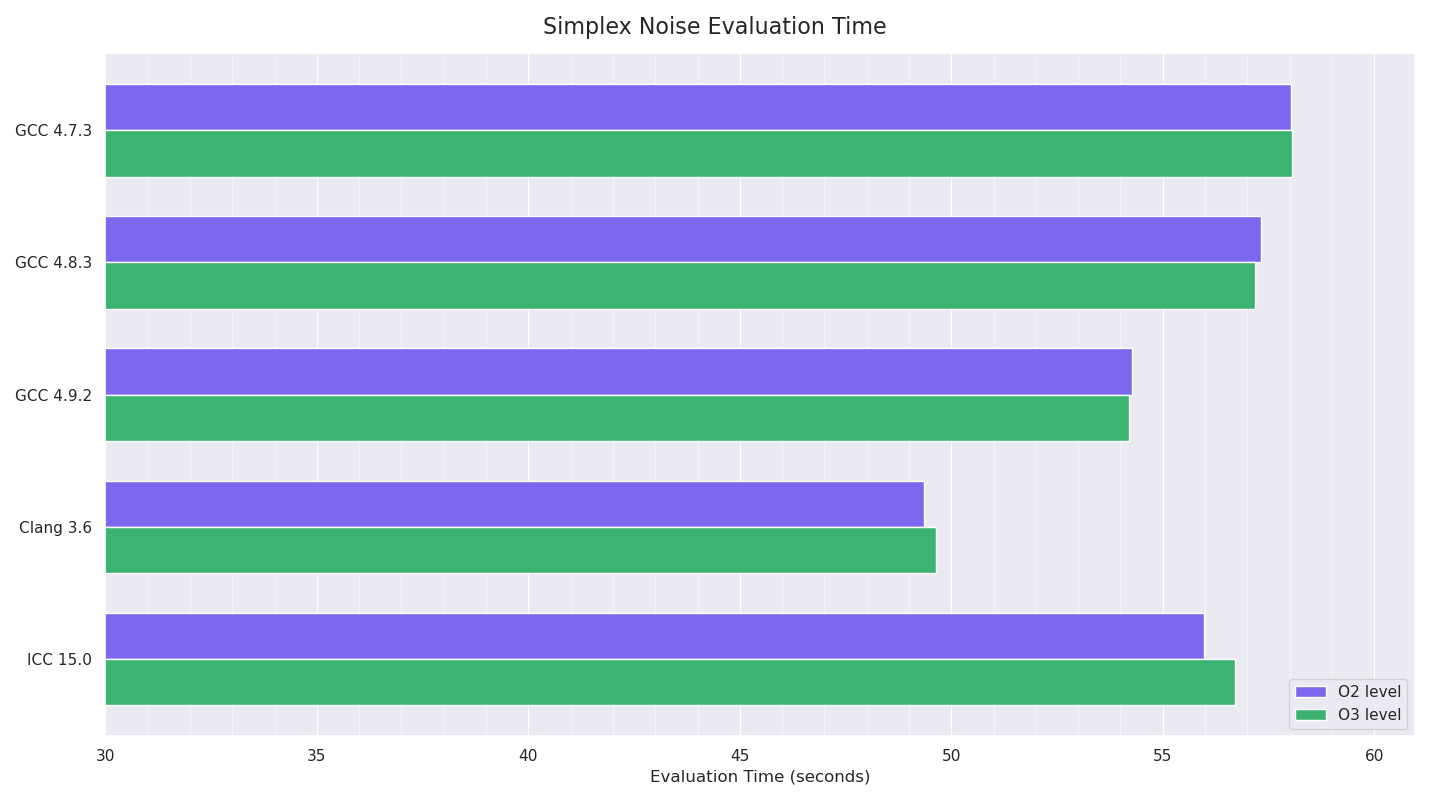
Recently, I had been about to upgrade my Linux distro on my main workstation at home, and this brought an upgrade to GCC 4.8 from 4.7 as the base GCC version. Before I upgraded the distro I tried building Imagine with 4.8.3 built from source, and needed to fix some template code as g++ 4.8+ (ICC has never liked it either) now doesn’t like using pure abstract classes as a template type. I made this change to the code, and did some quick approximate benchmarks between 4.7.3 and 4.8.3 which showed there wasn’t really any improvement, so I decided to try 4.9.2 which had just been released. This seemed to showed a fairly serious regression in terms of speed (speed being a pretty important aspect for a renderer), so I decided I’d do a more comprehensive comparison of the latest main compilers for the Linux platform, as back in 2011 and 2012 I used to do compiler benchmarks (GCC, Clang and ICC) regularly every six months or so on my own code (including Imagine), and on the commercial VFX compositor made by the company I worked for at the time, and it had been a while since I’d compared them myself.

I’ve never really liked just doing micro-benchmarks/synthetic benchmarks of just loops, etc of simple code, as they can paint a distorted picture of what’s going on, which can’t always be realised when the same code is put in context within other code - a good example of this is C++ virtual function overhead, which I’ve previously benchmarked, and while it’s possible to see overheads in micro-benchmarks, the same code within an actual real application shows no issues (at least in my particular usage of them) - so I always try to benchmark code doing what it was designed for from a user’s perspective: in Imagine’s case, this is rendering, or aspects related to that.

As it stands now, Imagine consists of over 164,000 lines of C++ code (including comments) in 386 .cpp files and 484 .h files, included heavily (more-so than I’d like, as it causes pretty severe final binary code bloat) templated code for everything from the acceleration structures, image texture / filtering infrastructure to geometry attribute / indices / triangle type code and a fair amount of SSE intrinsics usage for some of the acceleration structures, image filtering, procedural noise textures and triangle packet intersection code. The rest of the code is standard 2003 C++ - GCC 4.1.2 is still used heavily in the VFX industry (due to plugin ABI compatibility issues), so I still want to be able to build Imagine with this compiler if need be. Other than (optional) image library libs (OpenEXR, libpng, libtiff, libjpeg) for file readers/writers, there are no other requirements/dependencies Imagine needs to build.

The compilers I eventually benchmarked were: GCC 4.7.3, GCC 4.8.3, GCC 4.9.2, Clang 3.6 (prerelease from SVN - with -enable-optimized configure option) and Intel ICC 15.0 trial. I did spend several hours trying to get GCC 5.0 prerelease built from SVN, but gave up after I couldn’t get it to accept either my system zlib installation or a custom one I built from source - googling seemed to indicate this was a multilib compatibility issue and I could get around it by symlinking include and lib directories for various things, but doing that didn’t work for me. I also wanted to compare earlier GCC versions, but couldn’t get 4.6 or 4.4 to build from source on my system either - again, seemingly due to multilib issues.

Comparing compilers fairly is a difficult thing to do as they all have different abilities in terms of optimisations, and even for the built-in standard -O1/-O2/-O3 optimisation types, they do different things for these. However, given the huge amount of different options they have controlling things like inlining aggressiveness and limits, loop unrolling, vectorisation, etc, it would be vastly time consuming to try every compiler option progressively to try and find the best combination for that version of compiler, although that would be the fairest test in terms of benchmarking the fastest code a particular compiler can produce for a specific set of limitations (instruction support, etc). For this reason, I’m going to stick to just comparing each compiler with both -O2 and -O3 with SSE4 support, as these are generally the starting points for using the compiler.

I decided to run three different rendering tests, each one testing slightly different features of Imagine, although there would obviously be a lot of overlap between the tests, and then two synthetic tests: one of image mipmap creation and the other of procedural noise evaluation.

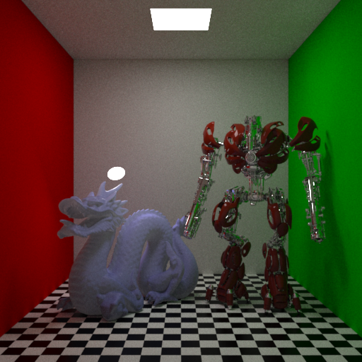
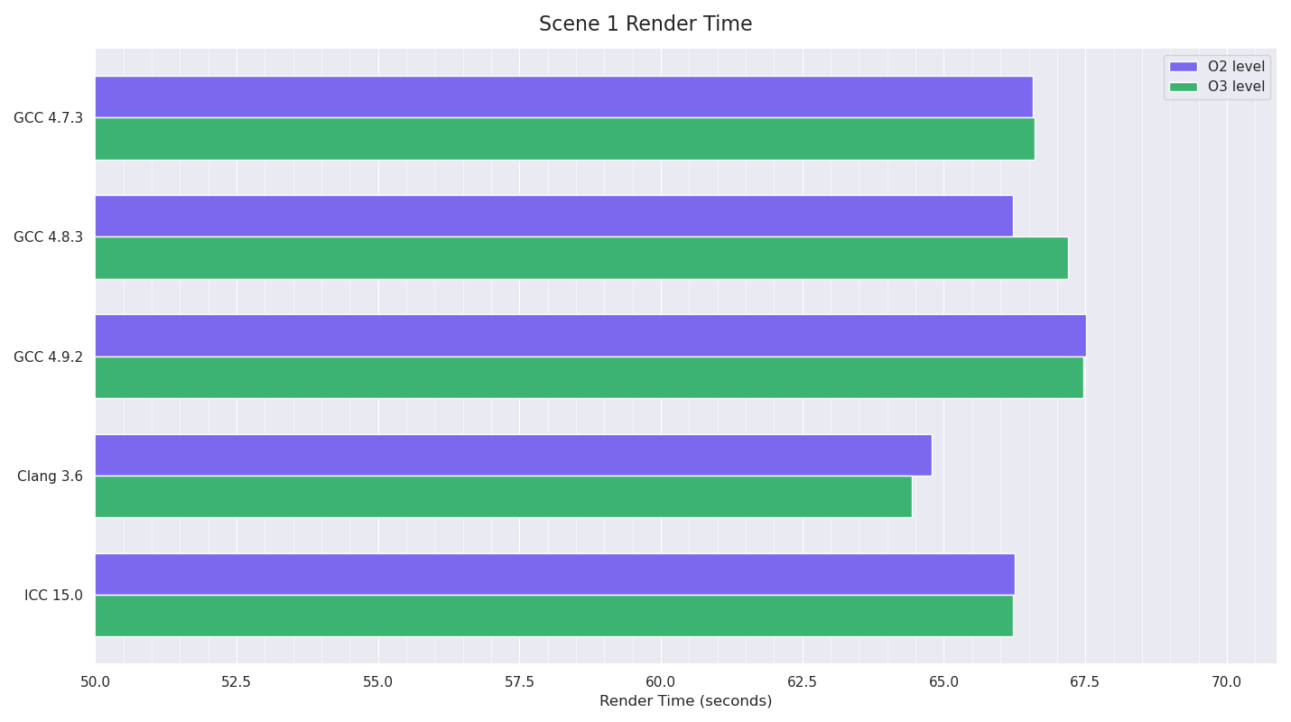
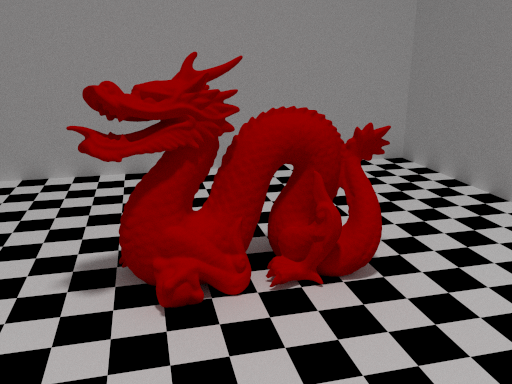
Scene 1 was a fully-enclosed cubic room, but with the front wall plane invisible to camera rays allowing them into the scene. Inside were the Stanford dragon at 1M triangles with a translucent SSS material, and the Katana robot example model with a combination of metal and car paint materials. Two area lights illuminated the scene, a standard ceiling quad and a disc light behind the dragon. This test made use of brute-force multiple-scattering volumetric integration for the SSS, with uni-directional path tracing with MIS, with two light samples taken per direct lighting evaluation. A total of 5 ray bounces were allowed, with a limit for diffuse and glossy of 4, and 5 for reflection rays.

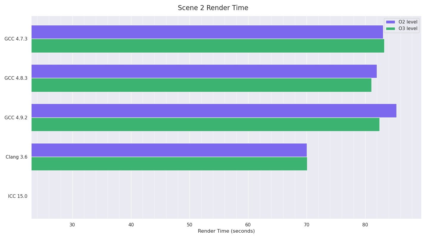
Scene 2 consisted of a large plane with a highly anisotropic metal material with a simple toy train model with diffuse, specular and bump textures and Cook-Torrance-style materials. There was also a volume primitive backed by dense voxel grids for density and temperature with a (pretty poor) blackbody shader for the emission colour based on the temperature. Trilinear interpolation was used to lookup voxel values. The last object was a toy helicopter with metal and plastic materials, with the rotors animated and quaternion interpolation used for motion blur. An HDR environment light was used. Brute-force multiple-scattering was enabled for the volumetric integration.

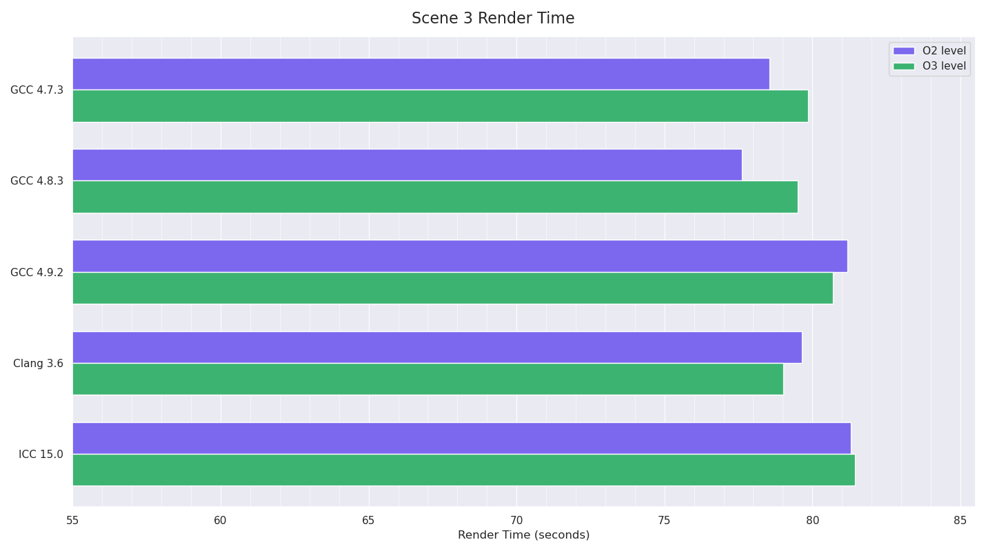
Scene 3 was an extremely large plane with reflective surface and a procedural bump texture, with an island mesh with 165,000 instanced trees on it. The trees had diffuse textures on the trunks as well as procedural bump textures (simplex noise), and the leaves were constant diffuse+backlit+CookTorrance spec, with an alpha texture for cut-outs (using stochastic presence sampling for all ray types). An HDR environment light was used. This was rendered as a Deep Image (alpha), so the integrator needed to do extra work collating and possibly merging each pixel sample for each pixel.

I configured Imagine to use completely deterministic sampling (the random numbers used to generate samples were consistent between runs per thread), and all textures were pre-loaded in memory before starting the renders. Similarly geometry processing and acceleration structure building was done before starting the timers, meaning these rendering tests should be completely deterministic in terms of calculations and would only be memory / CPU bound, essentially testing raytracing intersection, light integration, texture lookups, procedural texture evaluation, etc.

Compile flags used for GGC/Clang builds:

-O<n> -march=native -mfpmath=sse -fPIC -ffast-math -msse -msse2 -msse3 -mssse3 -msse4

for ICC builds:

-O<n> -fPIC -fp-model fast -msse4 -no-intel-extensions

(plus some experimental tests I later did with: -O3 -no-prec-div -fp-model fast=2 -xHost -inline-level=2).

My system was a dual-socket Xeon quad (E5-2643), with eight physical cores - 16 threads with hyperthreading (which I made use of for the rendering tests). Linux Kernel version was 3.5. Timings are mean averages over multiple runs, with the system idle and making sure all CPU core temps were under 45 degC to not bias things by allowing turboboost being used differently between runs.

Results

I did some quick compile timing tests (all using eight jobs only to make sure the build wasn’t IO constrained). Three runs of each from a completely clean build, other than for ICC which kept having FlexLM license errors, so I only had the patience to do two runs for ICC. Mean averages are shown.

To my surprise, Clang was slowest: generally I’d previously found that Clang was much faster at compile time than the other compilers, and other recent benchmarks seem to show that picture as well. Running single-threaded builds of Clang and GCC 4.7 showed similar results: 6 minutes 18 secs and 4 minutes 49 seconds respectively, so I’m not sure what happened here.

(Later Edit: it turned out I had built Clang with asserts enabled, which meant it was doing extra work, and meant the timing numbers for Clang for compile times using it were inaccurate, but all other results here are valid from the build).

For the three render scene tests, Imagine was started, pre-renders were done, I ensured all the CPU core temps were under 45 degC and the system was idle, and then I rendered the scene. Rendering was done with 16 threads (using full hyperthreading of the machine), and each thread had its affinity tied to a unique CPU id (using pthread_setaffinity_np()), hopefully meaning there was less scope for the scheduler to bounce threads around different cores leading to cache misses (in the past I’ve noticed more than measurable speed improvements by doing this especially when the machine has multiple CPU sockets). Timing for just the rendering stage was printed to the console. I ran each test separately, restarting Imagine and doing the pre-renders each time (meaning memory for the images, geometry and acceleration structures would very probably be allocated in different places each time).

I did at least four tests with each compiler / optimisation level combination, often doing more when the variance between the numbers looked odd or too large. I saved the render output of two of each combination for checking later (to ensure they’d rendered the correct thing and to compare final output values).

The tests for Scene 1 had Clang as the winner by a fair margin, with GCC 4.9 very slightly slower than the previous GCC versions. Only in Clang’s case was the O3 build noticeably faster than the O2 one.

The tests for Scene 2 also seemed to have Clang as the clear winner, although I couldn’t run the Intel ICC tests as there were severe issues with the acceleration structure build code which only triggered in this test (code branches were being taken that shouldn’t have been possible). For the moment I’m putting this down to an ICC bug (given past experience with ICC, unfortunately it is pretty buggy) as marking a uint32_t class member variable as volatile “fixed” the issue, but it definitely seemed that ICC was emitting code that would not copy across all the bits of a uint32_t and so was truncating it, leaving some bits uninitialised. This code was only running when motion-blur was being used for an object (the helicopter’s blades in this case) - basically a special type of primitive clipping that works well with motion blur bounds. I added debug code to verify that none of the other compiler builds were doing things wrong in that place, and as I didn’t want to test ICC with this volatile modification which shouldn’t have been needed, I just skipped it.

GCC 4.9’s results however, showed that the timings were pretty inconsistent: ranging from 88.43 seconds to 82.39. I couldn’t find any pattern to this: the system was idle, CPU temp was down before starting, output results for all the different compilers matched almost exactly (the fast math option was enabled for all compilers, meaning the compilers weren’t required to always stick to IEEE float precision, and thus there were minor variations in the results of some of their calculations, but the differences of the final render outputs were extremely minor), until I discovered that doing successive renders with the GCC 4.9 builds with the same pre-render state gave much more consistent results. Given that all the builds were doing almost exactly the same thing (very minor floating point value differences as pointed out above), this pointed to data memory layout differences causing this, possibly even due to memory alignment issues, but more likely due to differing memory layouts of things like acceleration structure nodes, geometry, etc affecting memory pre-fetching or branch prediction in some way due to the code GCC 4.9 was generating. None of the other compilers showed this issue. The only other difference with the GCC 4.9 tests was that I had to set LD_LIBRARY_PATH to point to the GCC 4.9.2 install’s lib64 directory for a newer version of libstdc++.so.6 in order to run these builds. However I don’t think this was the cause of these timing inconsistencies as I tried running some of the other compiler executables with this modified LD_LIBRARY_PATH (and verified using LD_DEBUG=files output that this newer lib was being used), and the other compiler builds I tested still didn’t exhibit this issue.

Scene 3’s tests are a much more mixed bag with no outright winner, although the O2 builds of GCC 4.7 and 4.8 were the quickest. Again, GCC 4.9 showed varying results, and as before, using the same pre-render state and doing consecutive renders gave much more consistent results (which I didn’t include in these results).

Due to the fact these rendering tests were testing quite a lot of different things at once, and I was slightly concerned about the fact that the ICC builds couldn’t run Scene 2’s test, as well as the fact that ICC wasn’t winning any of the tests (when I last benchmarked the compilers over two years ago, ICC was consistently > 25% faster than the other compilers), I decided to turn my attention to more simple synthetic tests.

For the two synthetic tests, I stubbed Imagine infrastructure code into much smaller separate executables, with code just running in the main thread (still with affinity set). The Mipmap test involved opening 6 8K 16-bit half RGB scanline OpenEXR files from disk, keeping them in memory (at full 32-bit float precision after conversion) and repeatedly generating filtered mipmaps for these images, 11 times each in rotation (so effectively doing 66 mipmap generations). I only started timing after the images were loaded off disk and converted to 32-bit float format, so the benchmark should be CPU and memory constrained only (quite a few memory allocations).

In this test Clang and ICC lagged GCC significantly, with GCC 4.9’s O2 benchmark strangely slower than the other GCC timings.

The procedural noise test involved iteratively evaluating 3D simplex noise at regular intervals at positions in the shape of a cube (stepping in each dimension), for a total of 1,194,389,981 evaluations. I disabled the SSE intrinsics support I had for this code, so it was just pure float / int operations and branching, to see what the compilers could do. This test should be fully CPU-constrained.

Clang won this test by a fair margin, with GCC 4.9 next fastest and ICC followed. I was still really confused by ICC’s poor showing, and started experimenting with more aggressive compiler options: -O3 -no-prec-div -fp-model fast=2 -xHost -inline-level=2 allowing less precision, using all instruction sets the host processor supported and more aggressive inlining at the compiler’s discretion. Doing this knocked a few seconds off the timings for ICC, but I’m almost certain (but didn’t test) doing equivalent things for the other compilers would have done like-wise.

Two years ago, libm’s maths functions (definitely transcendentals like pow(), sin(), etc) were pretty bad in CentOS 4/5 (often to the point that using double precision was significantly faster than the standard float versions), so using ICC meant that it had the ability to replace these functions with Intel’s own optimised ones (which at the time were much faster than libm’s) and statically link them inside the executable. Analysing the symbols in the built executables for ICC and the other compilers showed ICC 15.0 was doing this: most maths symbols for the non-Intel builds were Undefined, with them pointing to GLIBC, whereas ICC’s builds had the symbols in the executable. So I can only conclude that either GCC and Clang have become much faster over the past couple of years, or libm’s maths functions are a lot faster than they used to be. Both of which I think are probably the case.

I’ll need to do some profiling to work out what’s causing the GCC 4.9 builds to be so inconsistent, as that appears to be why when I first benchmarked with GCC 4.9 it seemed slower. This isn’t the most comprehensive C++ benchmark, but I think it’s a pretty fair comparison given that the compilers were all limited to a relatively similar degree - while the different compilers do different things at their respective O2/O3 levels, they have the same intent in that they’re recommended starting points, and O3 might be too aggressive in some cases - and taking into account how time-consuming it would be to play around with all the different optimisation flags for the different compilers. I would though have liked to have got GCC 5.0 built from SVN and to also compare the compilers with whole program optimisation, link time optimisation and profile guided optimisation, and to see what benefits those options might have brought over the more standard optimisations.

KDTree Benchmarks

I’ve been meaning to do some benchmarks on KDTree building / rendering for some time, given that although I’ve arrived at a set of build criteria which generally give the best intersection performance, I’d never actually done comparisons of the pros/cons of the different variables when building KDTrees and their cost/benefit ratio regarding intersection performance, and had never seen any published comprehensive benchmarks of KDTrees which tested more than one or two variables at a time. I’m also unlikely to play around with KDTrees much more, as I have to some degree moved over to using SSE-optimised BVH acceleration structures which generally provide slightly better render times, but orders-of-magnitude faster build time, thanks to standard binning.

Caveats: First of all, these tests are of my implementation of a KDTree. In certain configurations, it’s very close to PBRT’s reference implementation, but I’ve optimised the traversal code to reduce branching, and added “Perfect Split” clipping and min/max binning approximation as options while building. I’ve also added inverse hashed mailboxing to ray intersection. However, there’s no guarantees as to the correctness of my implementation, although in testing against other renderers which use KDTrees, it seems highly competitive, and is definitely faster than PBRT’s implementation - ~2x faster with an Empty Bonus of 0.9, clipping and using inverse hashed mailboxing.

So while the following results are fairly comprehensive, there’s certain build criteria I didn’t bother testing, and doesn’t in any way test the variable of leaf node threshold size, which I’m pretty certain will have a strong influence on both build time and intersection time. In addition, due to the time it’s taken to accumulate the results, I’ve had to reduce the number of test scenes down to three from the planned six, which also means these tests could be more thorough. I also recorded acceleration structure size, from which - because I know the KDTree nodes are 8 bytes each - I can work out the number of nodes the resulting KDTree had. Unfortunately, I didn’t record the breakdown of interior / leaf nodes, which would have been useful. I’m not showing those numbers in these results, but I use them in the results section to analyse some of the timing numbers.

The results of acceleration structure build time are also slightly misleading, although still relevant - I’ve disabled multi-threaded building of the KDTree for a few reasons: first of all, it’s not a completely parallelisable problem, and while it definitely is possible to parrallelise KDTree building to a degree, depending on the criteria used for building the KDTree, different amounts of parallelism are possible. For example using “Greedy” n log n SAH splitting, each thread needs to compile its own copy of the list of edges, and this either requires a lot more memory or if you break the task down into separate chunks a merge-sort stage at the end. It also causes a lot of cache thrashing, generally limiting the scalability of multithreading. So while the build times are not realistic in terms of “wall clock” time (generally I tend to get 3-4x speedup from multithreading the KDTree builds), given that they are consistently single-threaded for all configurations and the render times are consistently completely parallel, it allows a consistent comparison of the cost/benefit ratio for building a KDTree in a particular configuration vs. the render time.

Testing methodology / criteria

The theoretical best way to test ray intersection performance of an acceleration structure tends to be by casting well-distributed rays at the centre of the acceleration structure from a sphere around it, simulating incoherent rays, in such a way that path tracing will produce off diffuse surfaces. However, I’d prefer to keep tests more practical, so I’ve decided to test different meshes by putting them into a fully-enclosed room which has diffuse materials and a single area light and time how long it takes to build the acceleration structure for the main test mesh and render the resulting image. The number of ray bounces for all ray types will be four, and the render resolution and number of samples-per-pixel will be the same for all tests: 1024 x 768 and 128 respectfully.

Instead of baking down all the triangles into one main scene acceleration structure, I’m going to use the two-level acceleration structure hierarchy I use for instancing, such that the scene has an acceleration structure containing all objects, and each object’s geometry instance has an acceleration structure of the triangle mesh. This allows me to only alter the configuration of the central test object’s KDTree, while keeping the other acceleration structures for the walls, floor, etc and scene constant. The acceleration structures for the wall, floor and ceiling will each only have two triangles anyway, so will immediately produce leaf nodes.

For building the acceleration structure, I’m going to test two different methods: min/max binning SAH approximation, and the standard “Greedy” n log n SAH version which PBRT implements. For both methods, I’m going to test always splitting on the largest volume extent axis vs. checking all three available axes. For the “Greedy” method, I’m also going to test the effect the “Empty bonus” value has, and what effect clipping triangles (“Perfect splits”) has.

The only variable that will be tested for rendering itself is enabling/disabling Inverse Hashed mailboxing.

Test Scenes:

I’ll be testing the following three scenes:

Scene 1: Stanford Dragon: 871K triangles, in axis-aligned orientation

Scene 2: Robot: 1.6M triangles, at 45-degree rotation to axis-alignment

Scene 3: XYZ Dragon: 7.2M triangles, axis-aligned orientation

Because of the fact I’m using a two-level hierarchy of acceleration structures, in order to test Scene 2 fairly with regards to the axis alignment rotation, I’ve re-baked out the mesh in world-space with a 45-degree rotation around the Y (up) axis, so that its triangles are rotated within object-space as well.

KDTree leaf node threshold size is always 6, and for min/max binning approximation, when the number of objects left to be split is less than 8192, I switch over to the normal “Greedy” implementation - otherwise, I’ve found that min/max binning does a pretty poor job of splitting at that level. Published papers on the min/max binning algorithm for KDTrees seem to show similar issues.

In terms of recording the specific times, this is being done within the code using gettimeofday() to record the respective start/end times, calculating the difference and convert it to double precision, giving a number in seconds. That number is rounded to 5 decimal places.

For all test configurations, I’ve run six independent tests in a clean state, and the results shown here are the mean average of those results, again rounded to 5 decimal places. For the last two tests of Scene 3, there were differences in time for some of the tests outside the margin of error, so I ran a few more tests for those. The tests were all run on the same computer (Dual Xeon, Sandy Bridge micro-arch), running Linux 3.5 kernel, and all test executables were built with GCC 4.7.1 with the same options. I also tried to ensure that the CPU core temperatures were below 60 degC before running each test.

Test Results / Analysis

Scene 1

With min/max binning approximation, build times are relatively fast (a fair amount of the time is taken up by the “Greedy” partitioning which takes over after 8192 triangles), and surprisingly, while checking all three axes instead of just the single largest extent axis takes longer, it doesn’t take three times as long, which is what I would have expected. I guess some of the time would be due to memory allocation, which when checking all three axes is only done once.

On the rendering side, the fact that all axes were checked while building seems to have very little effect in this case, indicating that the extra time penalty for building might not always be worth the effort. Enabling Inverse Hashed Mailboxing has a huge effect on render times, effectively reducing the render times to ~73% of their previous times.

With the “Greedy” n log n partitioning method, build times are more expensive, and the “Empty bonus” value, used when building to maximise - or cut away - empty space has a very big effect on both the build time and the render time. Based on the memory allocation numbers I noted, and thus the number of nodes in each KDTree, I can see that having a bigger empty bonus leads to deeper (and therefore bigger) trees, as expected, but also better rendering times. Checking all three axes gives slightly better render times with an Empty Bonus of 0.9, but worse render times with one of 0.5. Triangle clipping is very expensive at build-time in this test, and only provides slight speed improvements at render time.

Although faster to build, the min/max binning approximation cannot generate trees as well as the “Greedy” one, so render times are significantly faster with trees built with the “Greedy” method. Once again, Enabling Inverse Hashed Mailboxing significantly reduces render times across the board.

Scene 2

Min/max binning really struggled with this mesh, not really partitioning the triangles very well, and leading to very large leaf nodes (over 400 triangles in some cases) once the depth limit (35) had been hit. Checking all three axes gave barely detectable improvements at render time.

Again, Enabling Inverse Hashed Mailboxing has the same effect as seen previously.

Once again, with the “Greedy” partitioning method, build times are more expensive, but with this mesh, a more aggressive Empty Bonus value produced deeper trees with no benefit - I think this is down to the fact that the mesh has been rotated at 45 degrees to the axis alignment, leading to non-tight AABBs. This is backed up by the fact that the tests with “Clipping” enabled (which spatially clips triangles to test split criteria as well as clipping a node’s BB to its parent node’s, thus removing overlap) not only build faster despite doing more work, but have significantly reduced render times. Checking all three axes in the final test with clipping enabled is much more expensive at build time over testing a single axis, but gives a reasonable render time improvement.

Once again, Enabling Inverse Hashed Mailboxing significantly reduces render times across the board.

Scene 3

In this test with min/max binning, checking all three axes has a fairly moderate penalty at build time over checking only one axis and provides a very slight render time improvement. Enabling Inverse Hashed Mailboxing provides a significant render time improvement once again.

The “Greedy” partitioning method takes a significant amount of time to build with this mesh, sometimes taking longer to build than it does to render (although building is single threaded as I’ve disabled multi-threaded building). Except for a strange result with the test with Empty Bonus of 0.5 and checking all axis, which for some reason produced huge trees (based on the number of nodes allocated) but still with large leaf nodes, leading to slow performance, the same general picture appears, although this time the “Empty Bonus” variable has much less of an effect, as does the clipping and checking all axes. This is probably because with this mesh it is axis-aligned in general, and the triangles are extremely small. Based on the build-time penalty for clipping and checking all axes, the pay-off for build-time vs render time in this test doesn’t seem as worth it.

Inverse Hashed Mailboxing once again brings down the render times in all cases.

Conclusion

KDTree building is very expensive, especially with “Greedy” n log n building, but in all cases this generates faster trees for rendering than min/max binning approximation does. The “Empty Bonus” variable seems to have variable results, with more aggressive values giving deeper trees but faster render times for some meshes, but producing worse trees in other cases. With “Perfect Split” clipping enabled, build time is even more expensive, but with meshes that don’t have tight AABBs, seems to be well worth the extra work. Checking all axes doesn’t really seem to provide that much benefit, but with min/max binning, it’s possible to parallelise checking all three axes at once with SSE intrinsics, so the cost/benefit payoff is possibly there, although that’s not possible for KDTree building with the “Greedy” method or when spatially clipping triangles, so standard scalar code needs to be used, increasing the work that needs to be done.

Using Inverse Hashed Mailboxing provides no build-time penalty and significantly reduces render time in all situations.

Future investigation: Given how much better the results of KDTree building are with “Greedy” building, I’d be interested in what benefit using min/max binning over standard binning has with BVH acceleration structures, and whether the huge potential penalty for doing “Greedy” building with BVHs would provide any render time benefits.

C++ Virtual Function Overhead

I have recently been trying to change Imagine’s Acceleration Structure infrastructure to be more dynamic, allowing different objects and geometry instances to have different acceleration structures either automatically based on heuristics, or based on user-specification within the interface.

Imagine’s acceleration structures have for the past two years been implemented with the Curiously Recurring Template design pattern, which allows virtual function-like ability to some extent while enabling the compiler to inline the functions. I chose this way of doing things as I had assumed that Virtual Functions would have some overhead, despite previously doing some experimentation with Virtual Functions and surprisingly finding they don’t seem to have any overhead compared to fully-inline-able functions.

The “Curiously Recurring Template” pattern doesn’t easily allow a templated base class (for Triangles, Shapes or Objects in Imagine’s case) to be specified as a pointer and then the actual implementation to be instantiated as a derived templated acceleration structure, which is what I needed for this dynamic flexibility.

So I decided to do some more benchmarks to investigate any overhead again.

First of all, I tried a synthetic benchmark of just a simple for loop of 1,073,741,824 iterations, calling getHitObject() on the acceleration structure pointer. For the “Curiously Recurring Template” implementation, the pointer type was of KDTreeVolume<T>, the actual derived class and the object allocated for that pointer was of the same type. In the Virtual Function implementation, the pointer type was to AccelerationStructure<T>, the base class and the actual object allocated for the pointer was KDTree<T>, a duplicate of the KDTreeVolume<T> class but which used standard C++ virtual inheritance from the abstract AccelerationStructure<T> base class. The code was run in a single thread.

Eight pairs of runs were done, alternating each implementation, and I tried to make sure the CPU core temperatures were under 55 degC before starting each test to ensure that there was no disadvantage to be had by a core not being able to Turbo Boost overclock.

Other than the first two results for the “Curiously Recurring Template” implementation, the Virtual Function method seems very slightly slower, but this difference is within the margin of error. This surprised me, but given the simple test case, it’s possible that the processor’s branch-predictor was negating the overhead of the v-table lookup, and thus might not be showing the difference.

So I decided to do some more realistic general purpose rendering benchmarks with the two different implementations, to see if any difference could be spotted there.

I created a scene with a fully-enclosed room, with 32 cubes inside and 2 area lights, and all surfaces fully diffuse. All geometry objects had less than or equal to 12 triangles, so the acceleration structures would be very shallow and thus any Virtual Function overhead would not be dwarfed by the work each function was doing on the acceleration structure.

The first test was at 1024x768, with 256 samples per pixel, and 10 ray bounces. With this test, the getHitObject() function would be called 2,013,265,920 times (for each camera ray and each diffuse bounce ray) and the doesOcclude() function would be called 4,026,531,840 times, once for each light (no light importance sampling was used) for each surface evaluation. All threads were being used for rendering.

The above results are in minutes, and show that the Virtual Function implementation was consistently slightly faster. I decided to do these tests again with double the number of samples per pixel (to double the above numbers), and again the results were pretty much the same:

I’m still surprised by this, but I’m putting it down to either compilers being a lot more clever than they used to, or the inlined “Curiously Recurring Template” implementation creating bloated instruction size. Or more likely, the fact that things like cache misses, load dependencies and branch miss-predictions within triangle and boundary box ray intersection code hide any overhead there may be.

Regardless, it appears that to all intents and purposes in my use-case, Virtual Function overhead is practically non-existent. I’m sure things would change with deeper inheritance hierarchies and multiple inheritance, but at least in my use-case it seems safe to move back to Virtual Functions. What’s more, Intel’s Embree high-performance ray tracing kernels use Virtual Functions, and they’re pretty-much state-of-the-art.